Getting Started Guide

Overview

The xVector Getting Started Guide is a hands-on guide for analysts and data engineers new to the xVector Platform. It walks through the end-to-end process of building a simple data app, from connecting raw data sources to enriching datasets and delivering interactive dashboards.

The business case used for the guide focuses on auto insurance churn data. Insurance companies lose revenue every time a policyholder cancels, and acquiring a new customer costs far more than retaining an existing one. Understanding who churns and why gives Account Management teams an early warning signal they can act on before a customer is gone. This guide uses three linked datasets, policyholder records, individual demographics, and suspended dates/accounts, to identify which customers are most likely to cancel their policy. It combines historical policy data, including tenure, premium amounts, and geographic attributes, with income, household composition, and credit quality to understand the financial and demographic profile of churned customers and surface high-value retention targets.

Before You Start, Download Your Data

Download the CSV files below and save them on your local machine.

File	What it contains	Role in this guide
customer.csv	One row per policyholder: policy details, age	Primary, your main source of facts
demographic.csv	One row per individual: income, education, credit, home ownership	Reference demographic data you will join with customer data
termination	One row per individual: termination dates	Churn data for customers

The files share a common identifier, INDIVIDUAL_ID, which is how you will connect them.

What does the data look like?

customer.csv sample columns and rows:

INDIVIDUAL_ID	ADDRESS_ID	CURR_ANN_AMT	DAYS_TENURE	CUST_ORIG_DATE	AGE_IN_YEARS	DATE_OF_BIRTH
221303009292	521301238852	936.44	6291	2005-09-11	76.97	1946-01-01
221301914491	521300694144	1529.67	4904	2009-06-29	40.31	1982-08-22

demographic.csv sample columns and rows:

INDIVIDUAL_ID	INCOME	HAS_CHILDREN	MARITAL_STATUS	COLLEGE_DEGREE	GOOD_CREDIT
221300017872	22500	1	Married	1	1
221300134410	27500	0	Single	0	0

termination.csv sample columns and rows:

INDIVIDUAL_ID	ACCT_SUSPD_DATE
221302577308.0	2022-10-09
221302825760.0	2022-04-24

Step 1: Create a Workspace

Before you can bring in data or build anything, you need a home for the project. In xVector, that home is a Workspace, a shared canvas where every resource associated with the Data App lives: datasources, datasets, models, reports, and agents. Workspaces make it easy to keep related work organized and to collaborate with teammates who need access to the same data and insights.

Follow the steps below to create a workspace.

1. Log in to xVector. This is your Home Page where you will see all the resources you have access to.

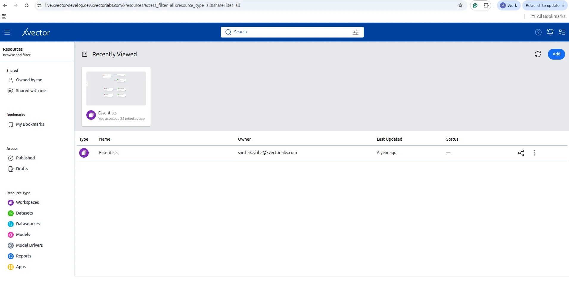
When you are first set up, you won’t see any resources. The right-hand side of the pane will be empty.

2. Click on Add (top right corner). Click on Workspace from the options list.

3. Update the Name: AutoInsurance_Churn

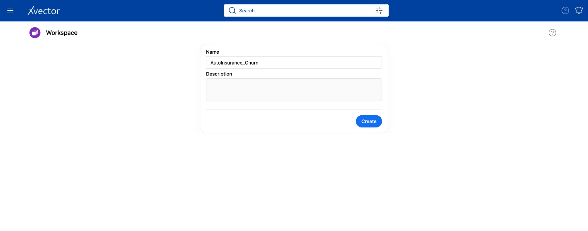
4. Click. Create.

You land on an empty canvas. Everything you build in this guide will appear in the workspace as tiles.

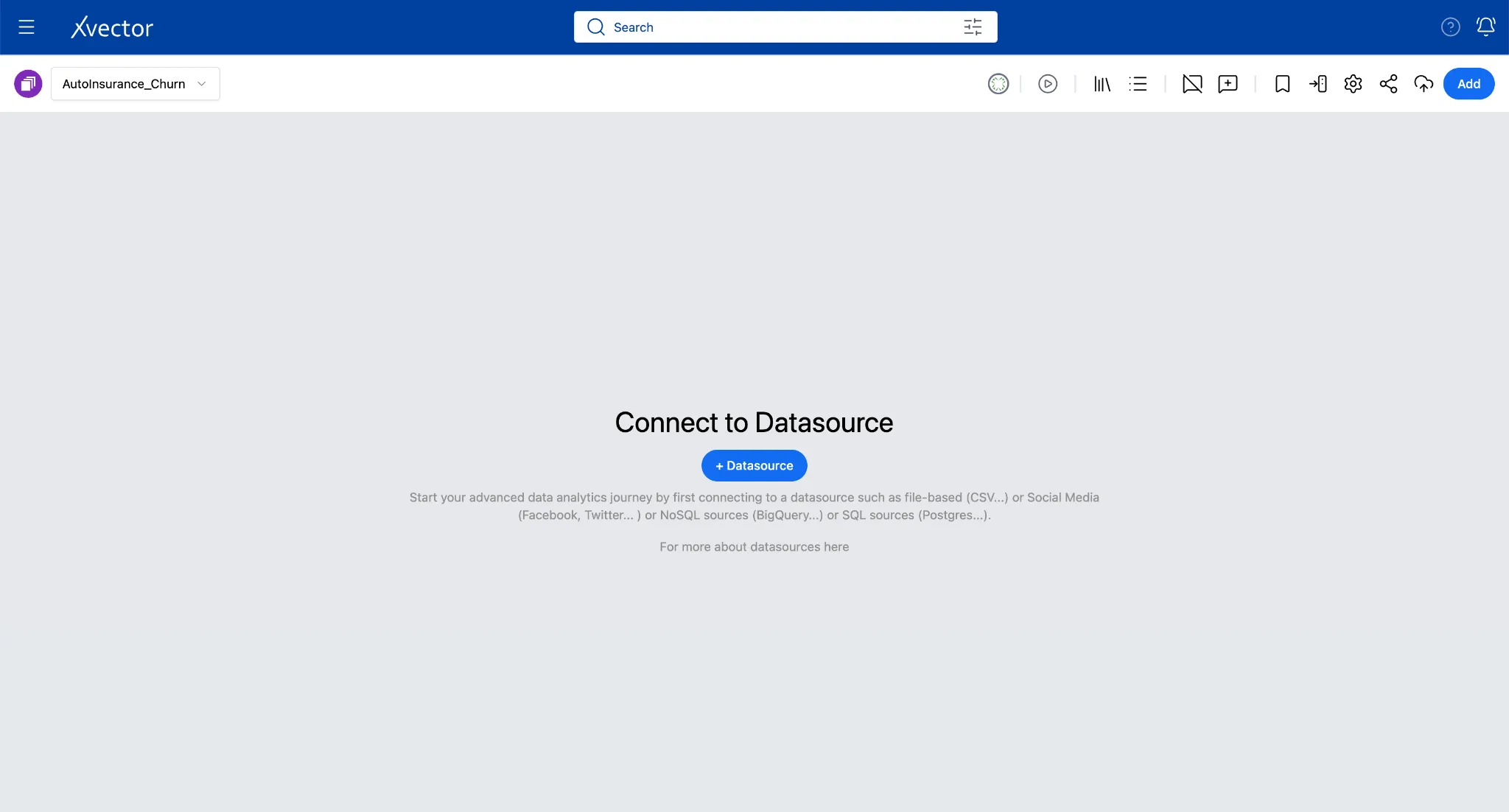
Start the Draft Driver before doing anything else

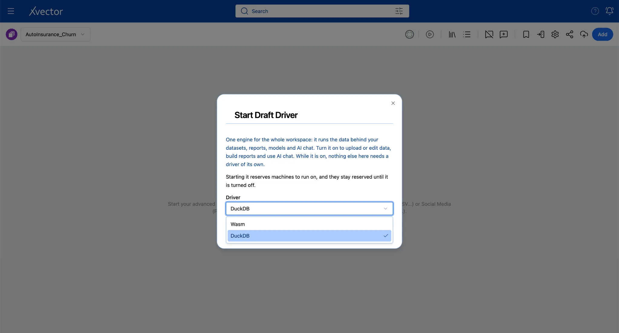
Click on the play button icon in the workspace toolbar. Draft driver can be started only from the workspace.

From the dialog box below, choose the DuckDB driver from the Driver dropdown menu.

And click the Start Driver button.

Once it’s up, a green dot appears.

The driver must be running before ingesting the data or performing any DML actions. The draft driver lets you experiment quickly.

Step 2: Import Data via Connectors

In xVector, a Data Source acts as a digital twin of your enterprise source system, where the connector imports the data from the source system into the platform seamlessly. While xVector provides a comprehensive catalog of built-in connectors and supports custom connectors for unique sources and formats, this guide focuses on importing data from your local filesystem using the CSV connector.

2a. Import customer.csv

customer.csv is your primary data source that captures the outcome you are trying to understand. Each row represents a single policyholder and includes policy details and age.

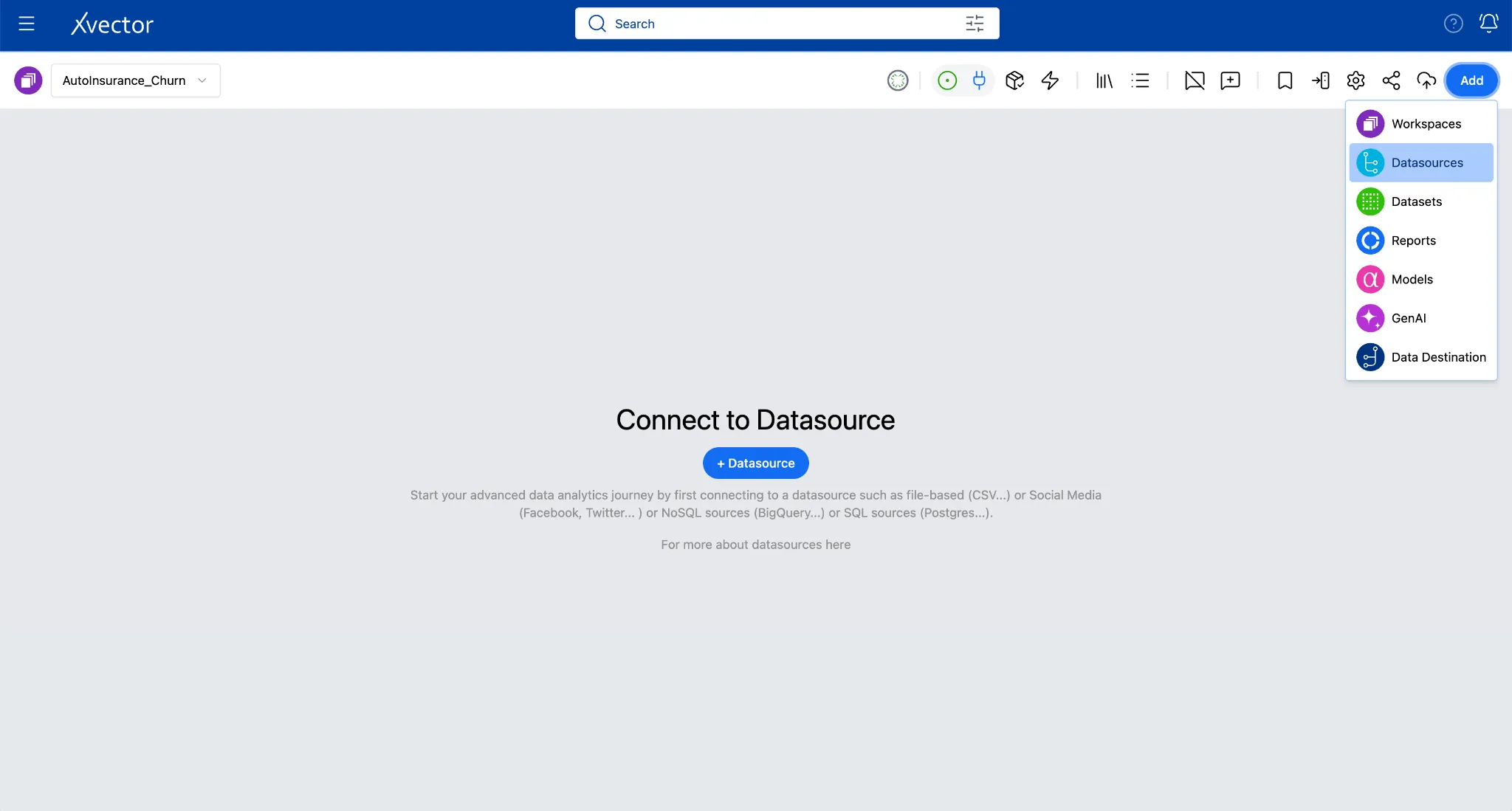
1. From the workspace canvas, click Add (top right) and choose Datasources, or click on the Datasource button on the canvas.

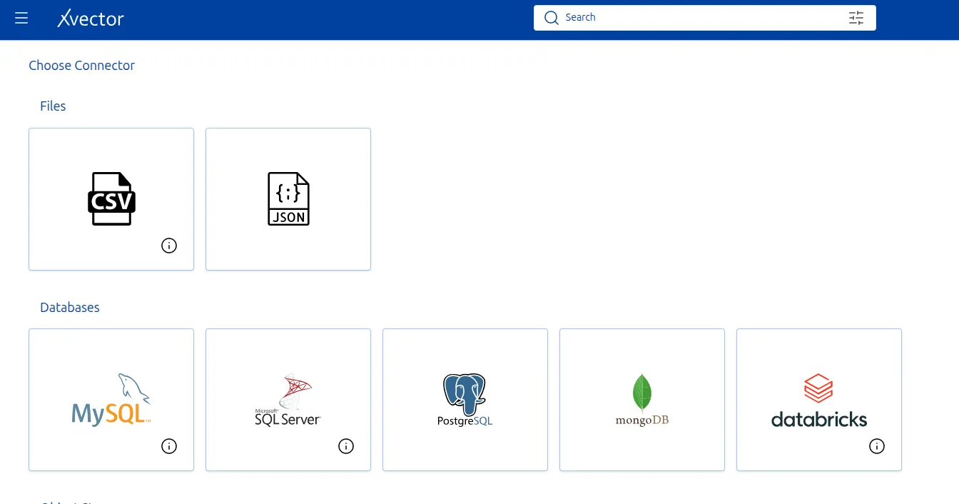
2. Select CSV from the connector list.

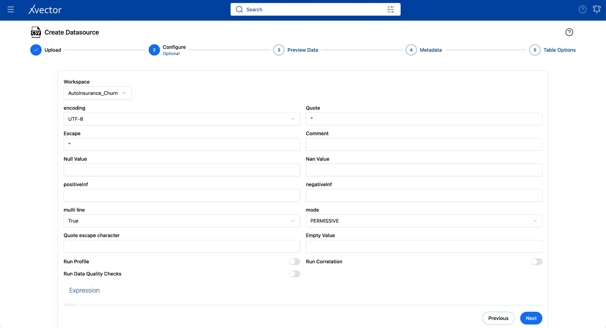
3. Fill in the Configure step:

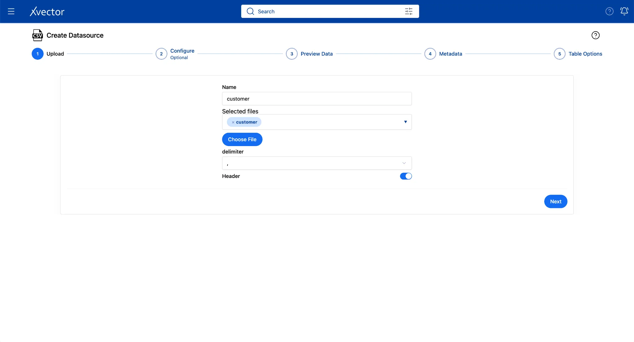
Below are the values for this example. You can add a Name of your choice.

Field	Value
Choose File	Browse to customer.csv
Name	Customer
Delimiter	Comma (,)
Header	True (default)

4. Click Next

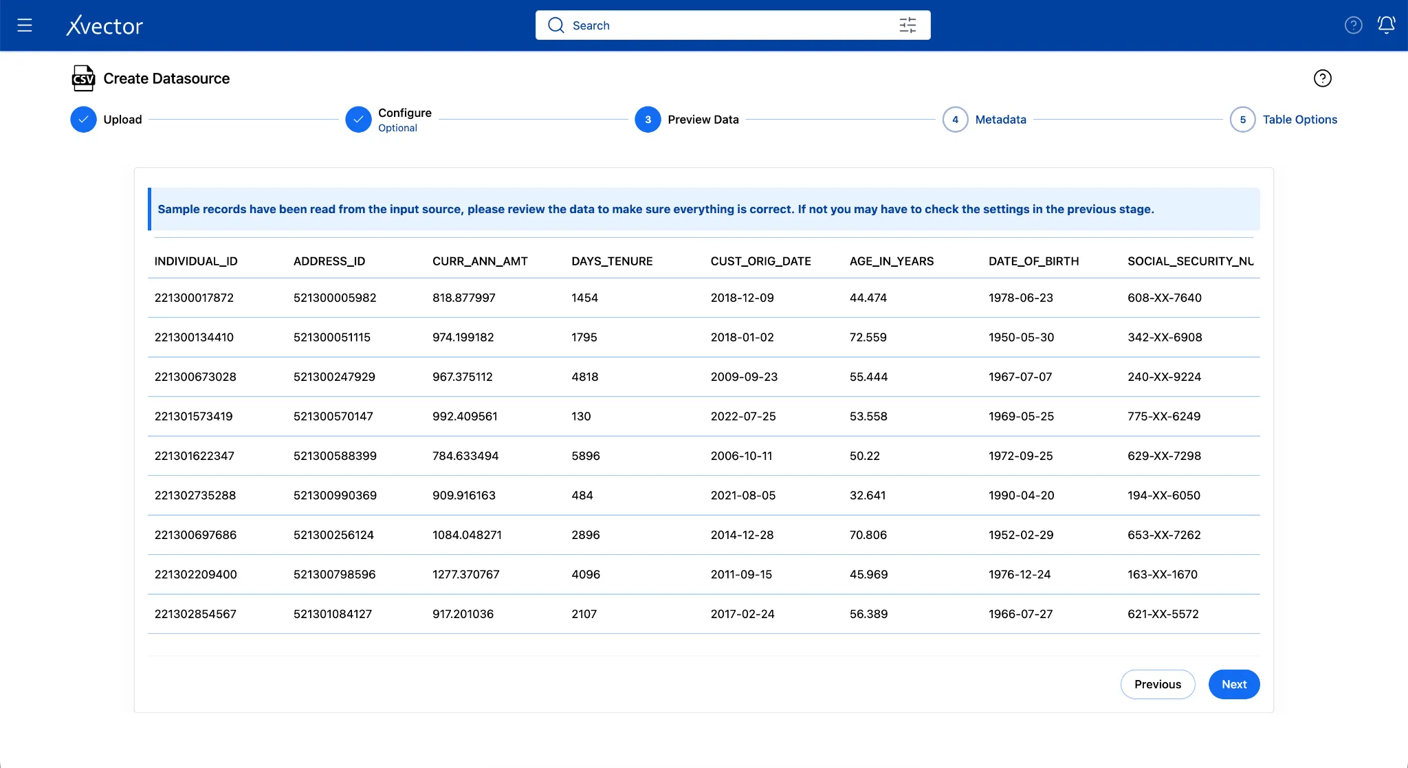
5. On Preview Data, verify the columns and click Next

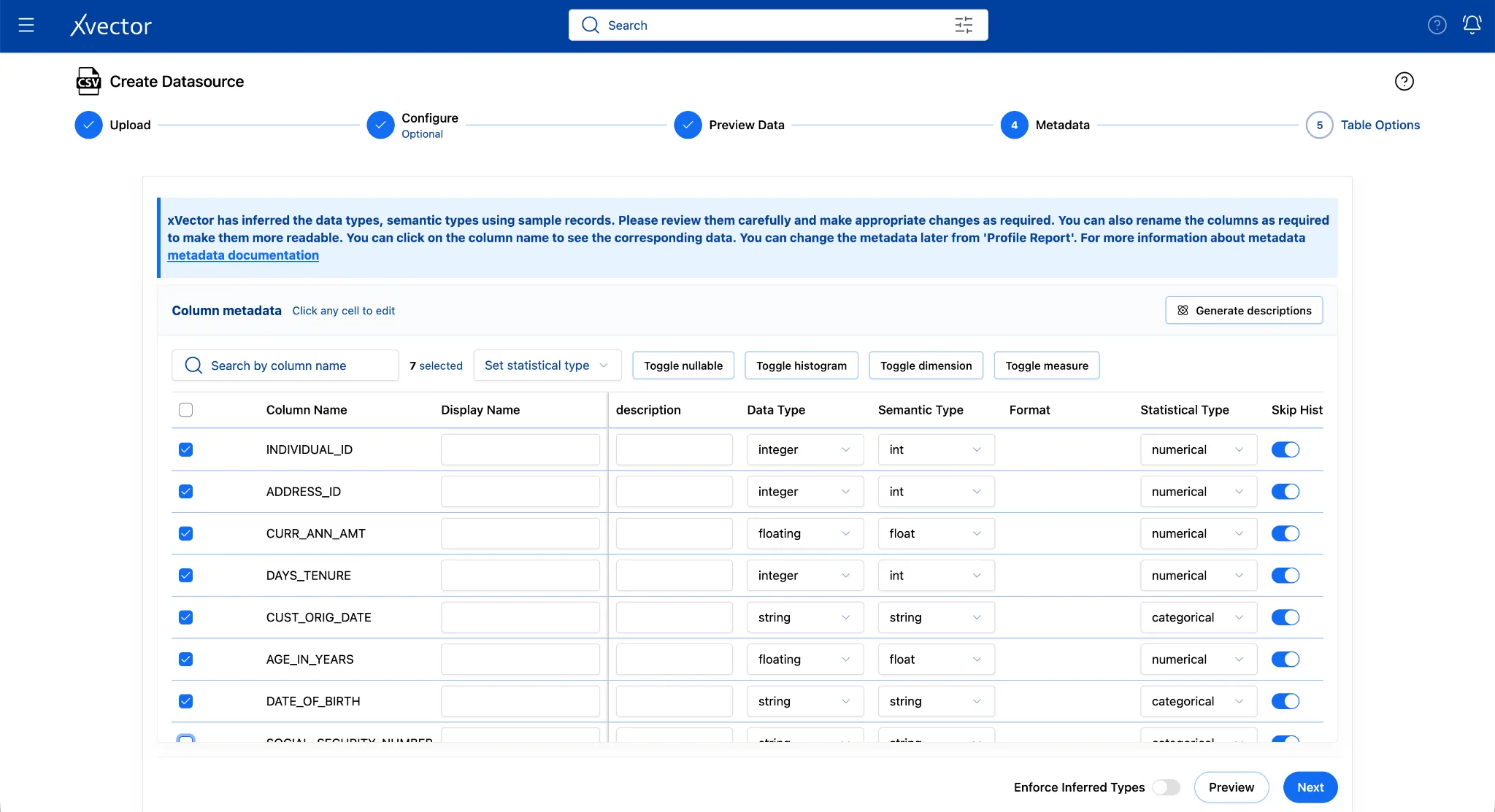
6. On the Metadata page, review Data Types, Semantic Types, and values in other columns. “Enforce Inferred Types” (bottom of the page) is turned off by default; keep it as default. This lets the data types update after the entire dataset is ingested instead of being inferred at the beginning. You can turn it on if you know exactly what the data types should be and you want to bring in the data with those data types.

Let’s say we don’t want to bring in the “Social Security Number” column since it is supposed to be confidential and it was being sent accidentally. We can simply uncheck the column in the metadata page.

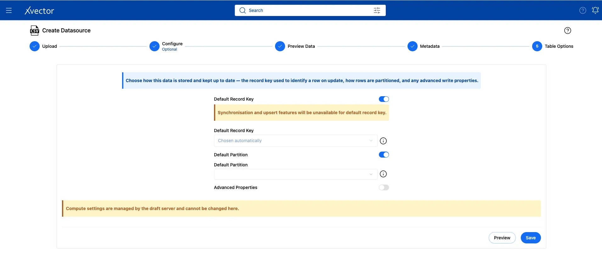
7. Leave the default settings for Table Options and click Save.

8. Click on Workspace once you see “Successful” in green.

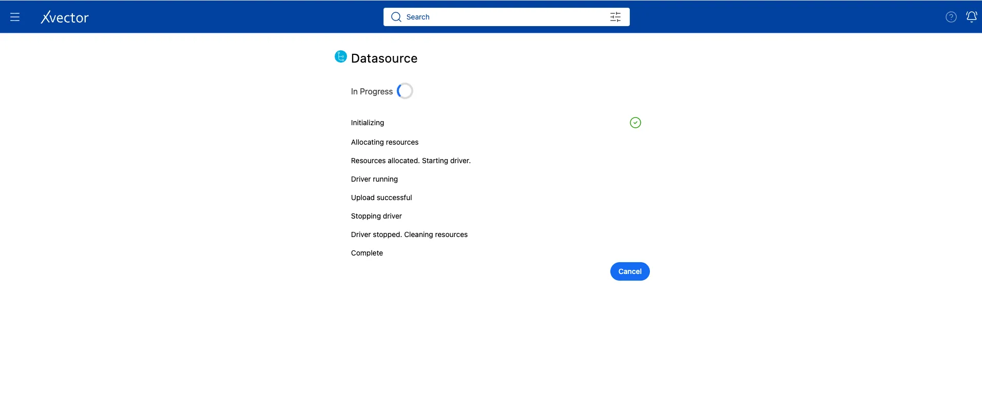
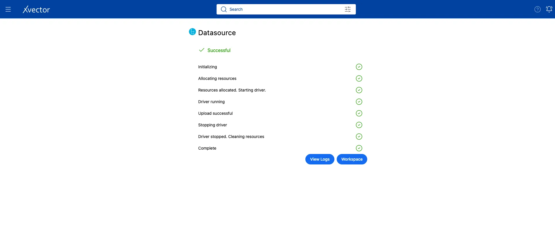
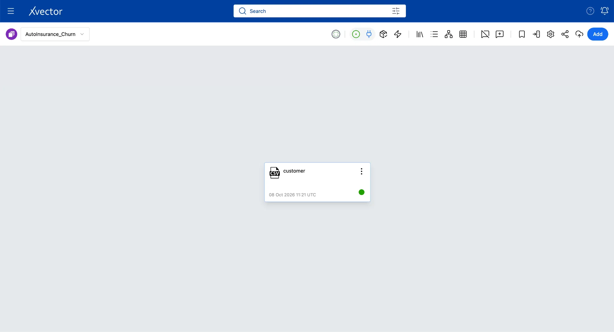
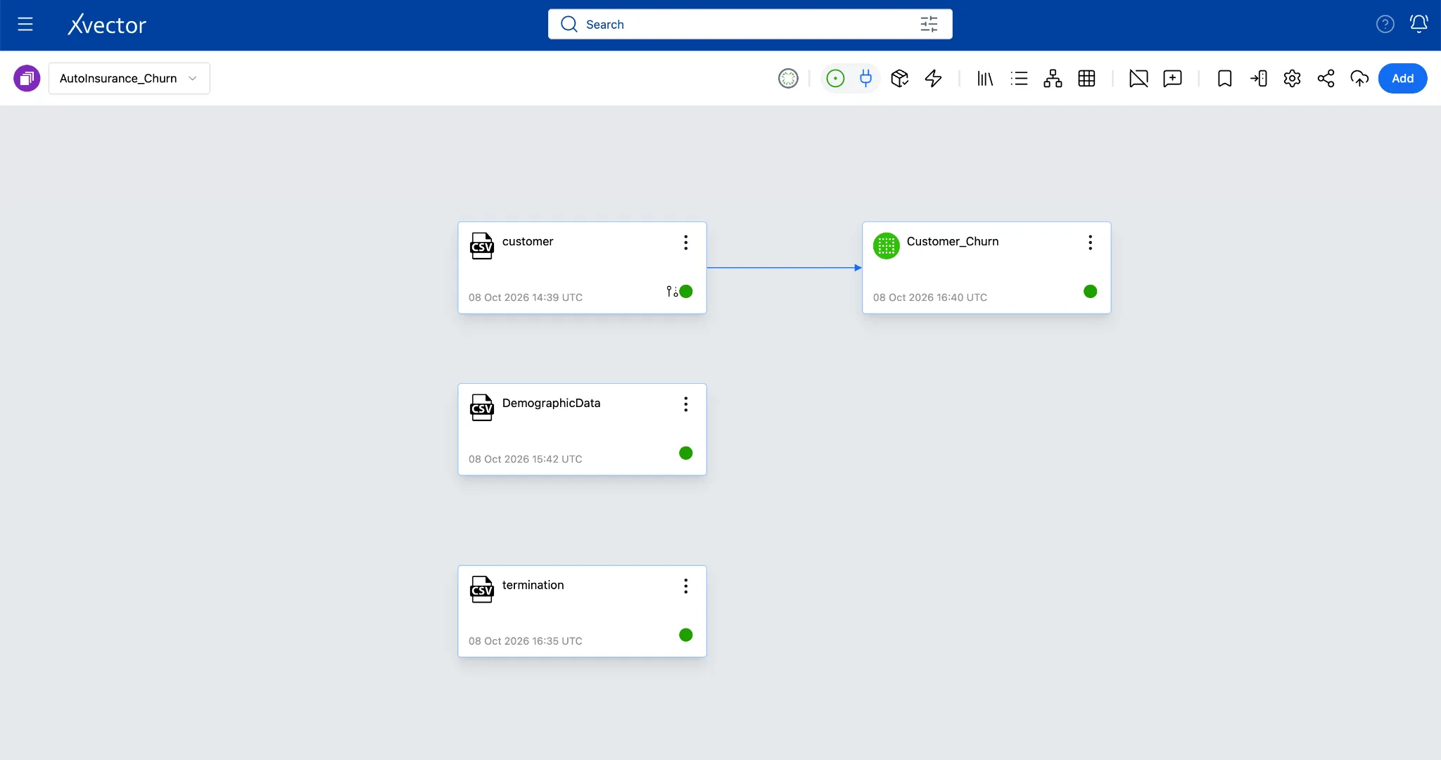
9. It will navigate back to the AutoInsurance_Churn workspace and show the Datasource created: customer.

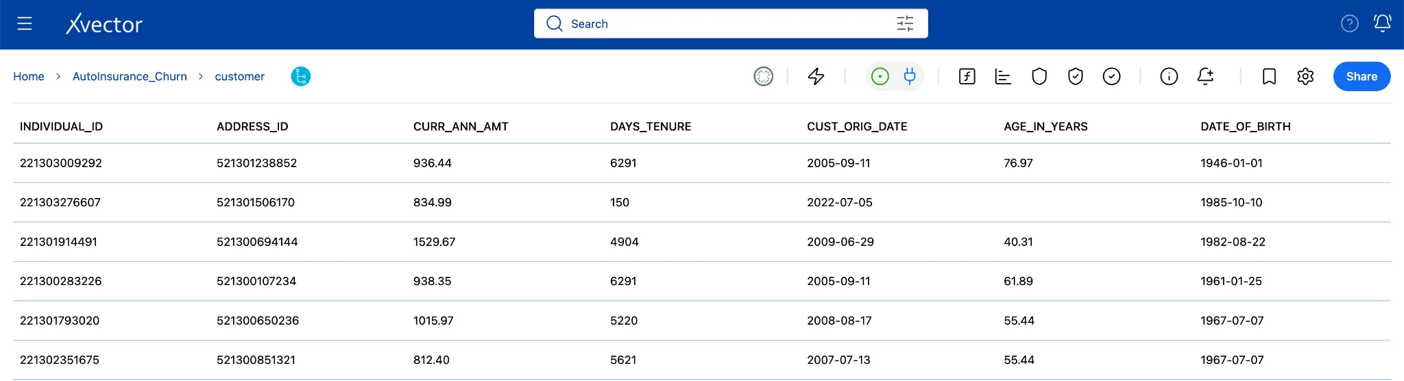
Double-clicking the customer tile gives the following view:

2b. Import demographic.csv

The demographic dataset tells you what happened but not who the customer is. The demographics file fills that gap. It holds income, education, homeownership, and credit quality for each individual, keyed to the same individual_id. On its own, this data is a static reference table. When joined with the churn data, it becomes the layer that turns a churn flag into an explanation.

Follow the same steps as in step 2a to import the datasource.

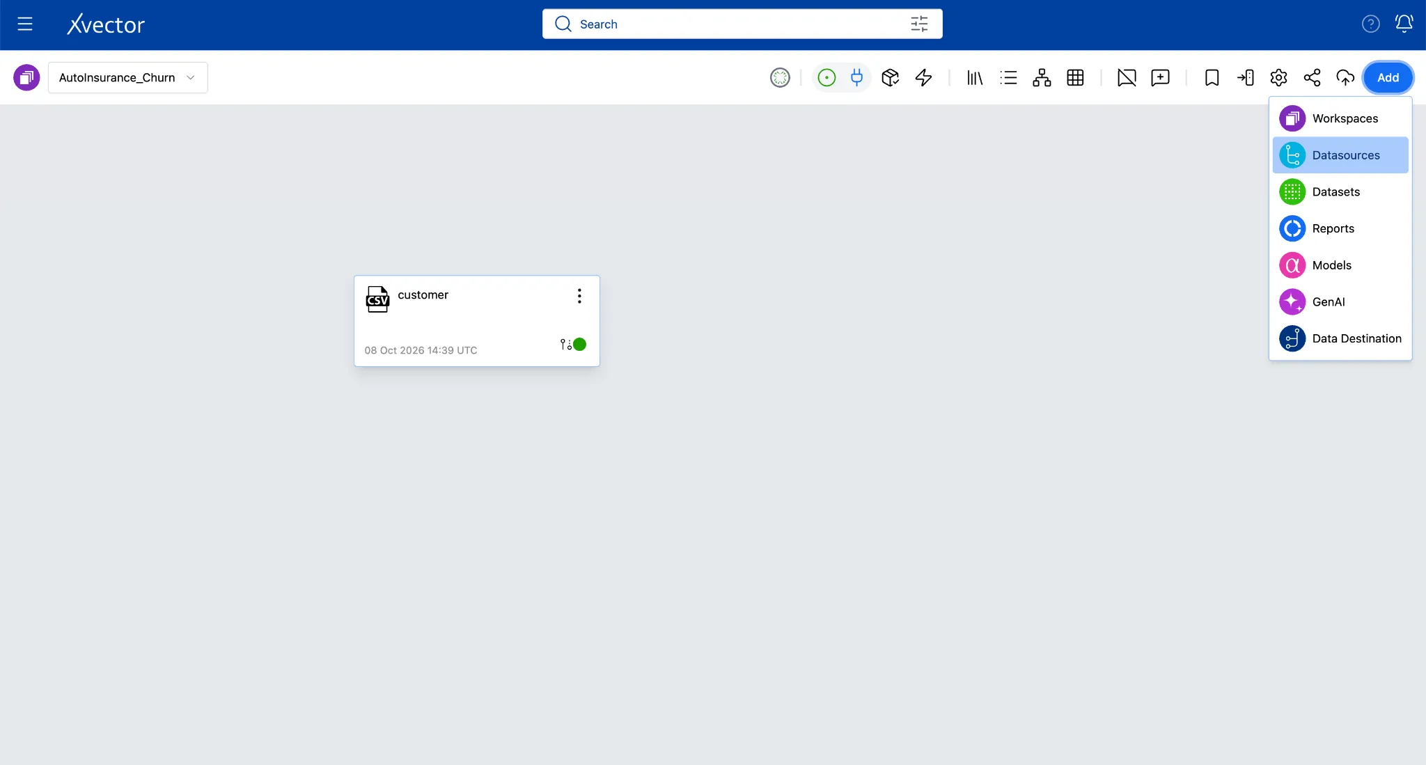
1. Click Add in the workspace, then Datasources, then CSV.

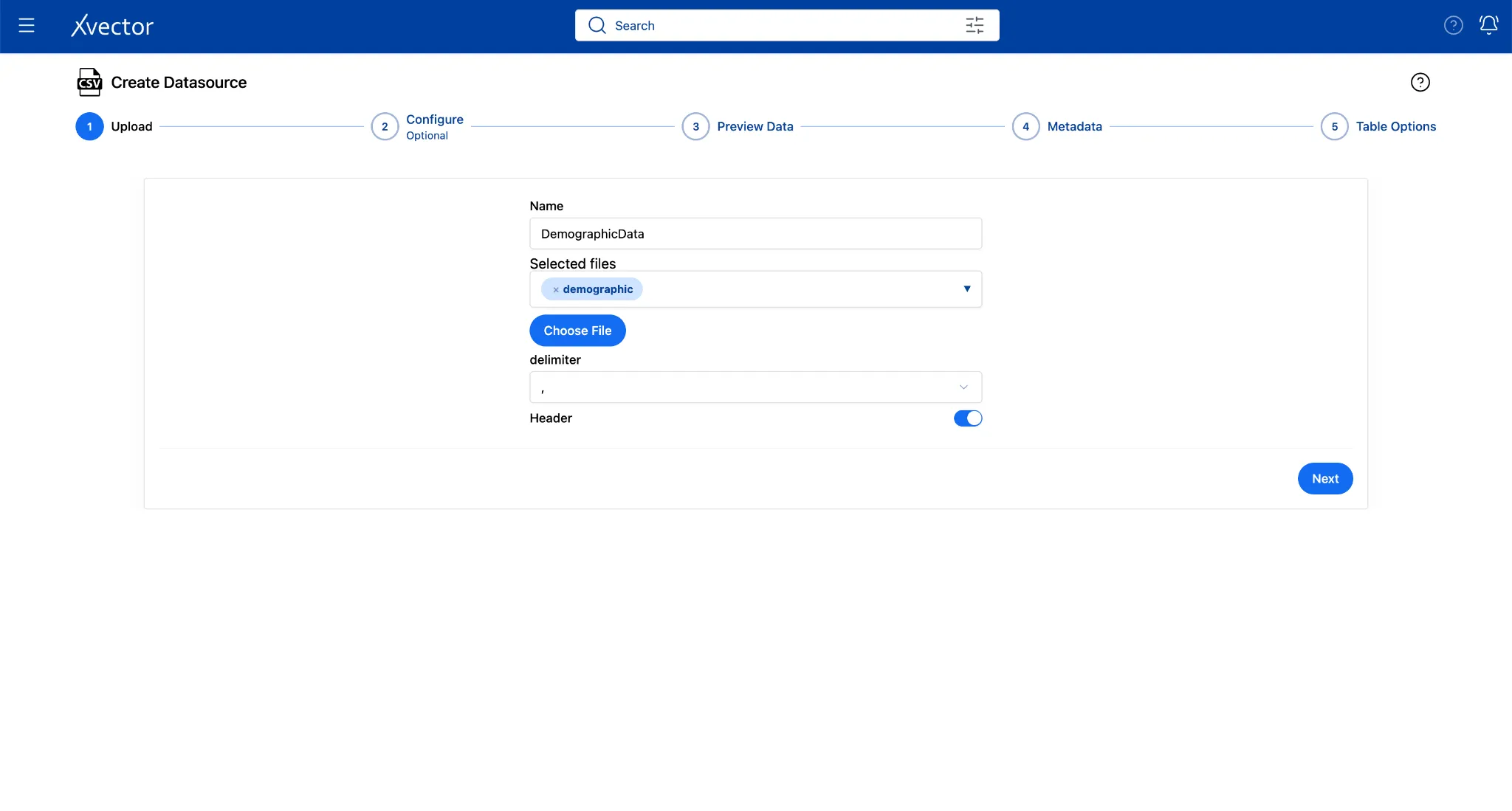
2. Fill in the Upload step:

Field	Value
Choose File	Browse to demographic.csv
Name	DemographicData
Delimiter	Comma (, )
Header	true

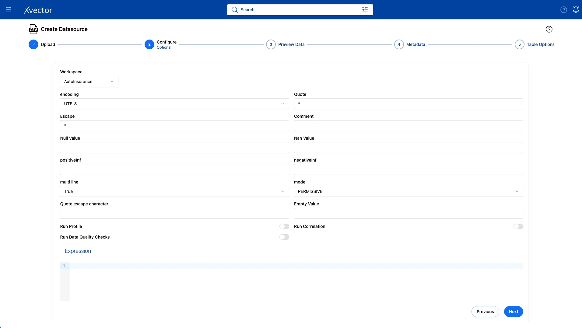
3. In the configure step, keep the defaults.

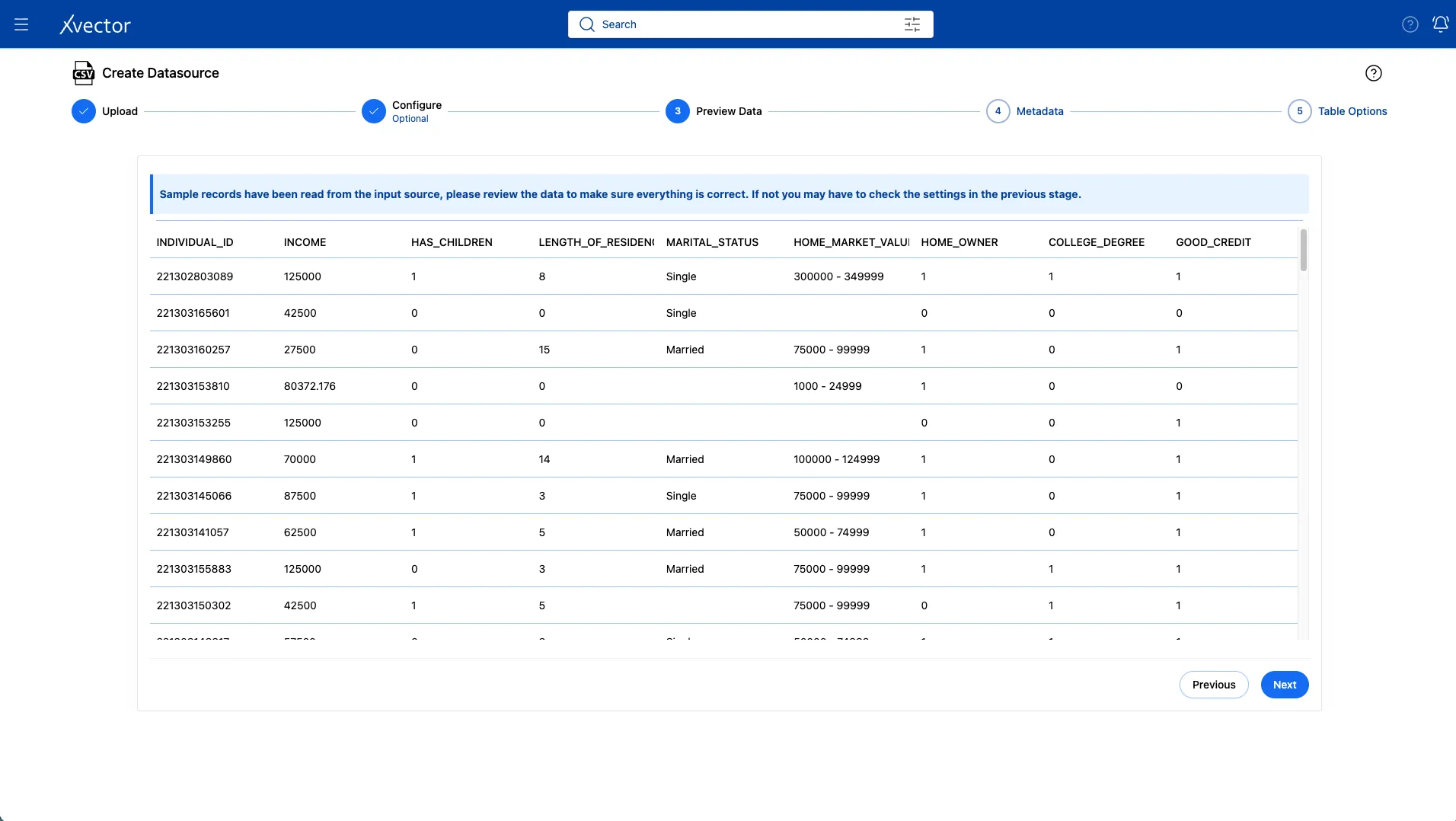
4. In the Preview Data page, you should see the columns: INDIVIDUAL_ID, INCOME, HAS_CHILDREN, MARITAL_STATUS, COLLEGE_DEGREE, GOOD_CREDIT.

5. In Column Metadata, find INDIVIDUAL_ID and rename it to individual_id (all lowercase) as the display name. This isn’t required, but it helps keep things consistent. We will join the 2 tables using this as the primary key.

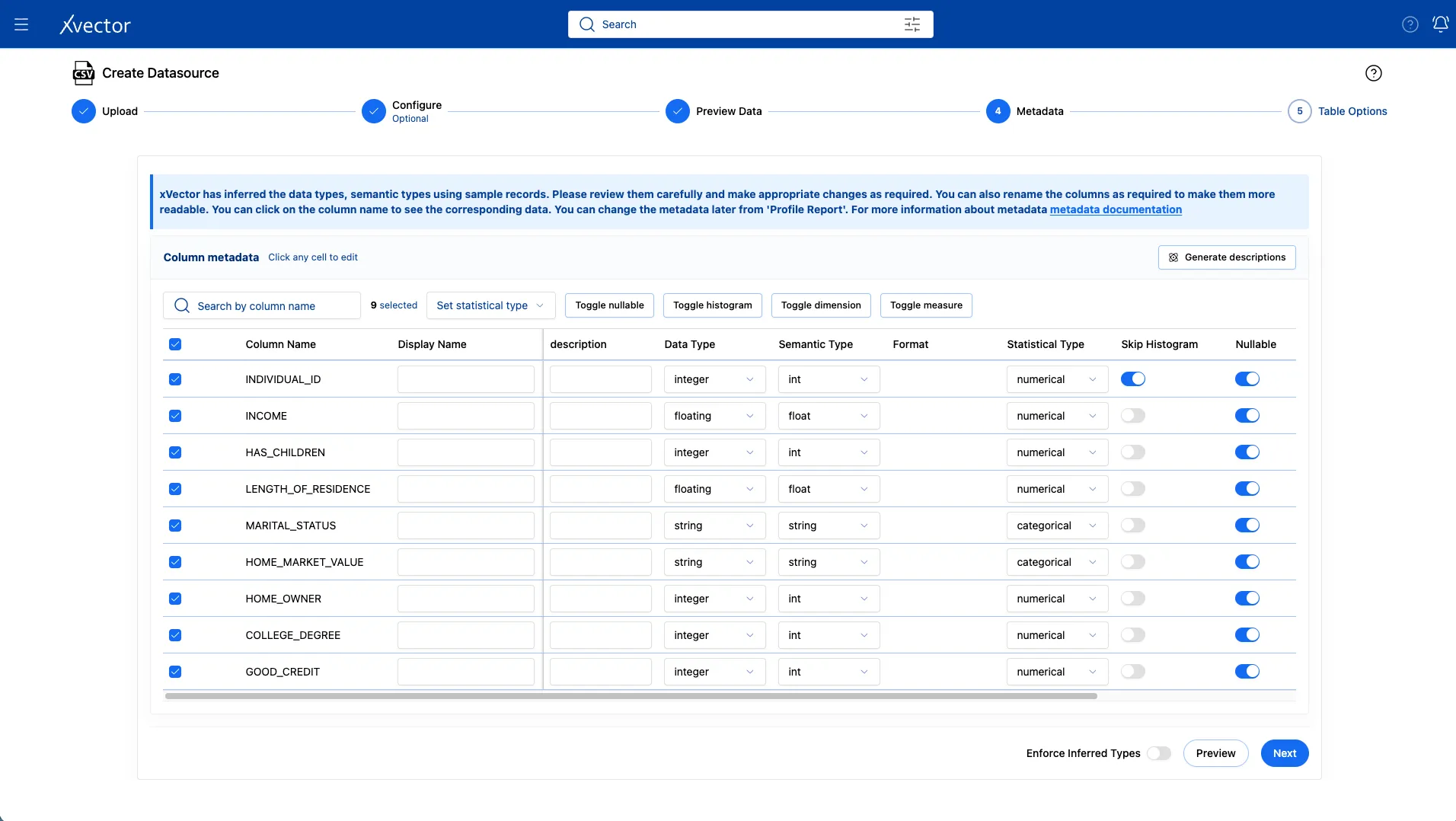
6. Leave the default settings for Table Options and click Save.

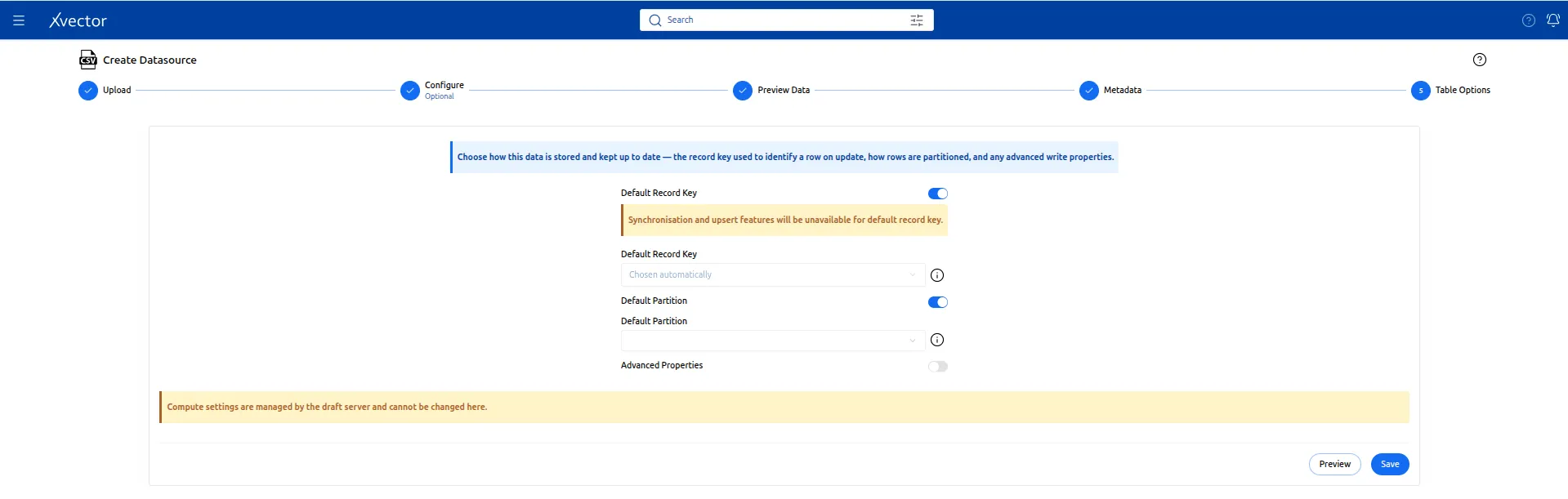
7. Click on Workspace once you see “Successful” in green on the screen.

2c. Import termination.csv

The termination dataset tells you when the customer canceled the insurance. This is what indicates the churn. Customers in this file are the ones who churned.

On the upload page, use the following:

Field	Value
Choose File	Browse to termination.csv
Name	termination
Delimiter	Comma (, )
Header	true

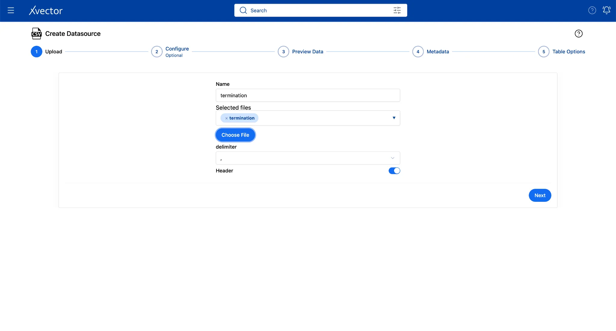
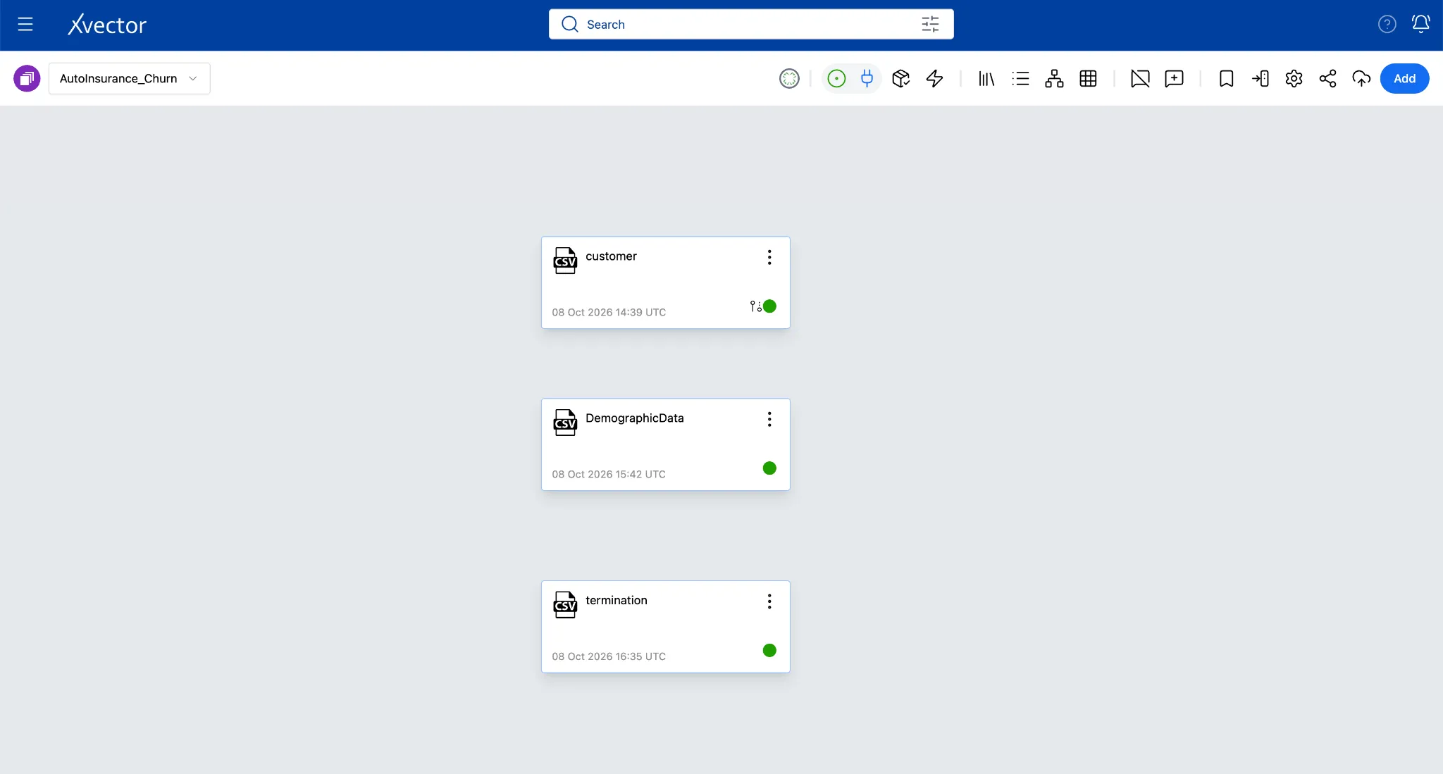
Step 3: Create Your Working Dataset

With both datasources ingested, you are ready to create the dataset where the real analytical work happens. Raw datasources are a digital twin of the enterprise systems. Datasets let you layer transformations, filters, joins, new columns, and many other enrichment functions on top without ever touching the source file. Every change appears in the xFlow Actions pane, so users can track exactly what was applied and in what order.

Now, let’s create a dataset from its datasource.

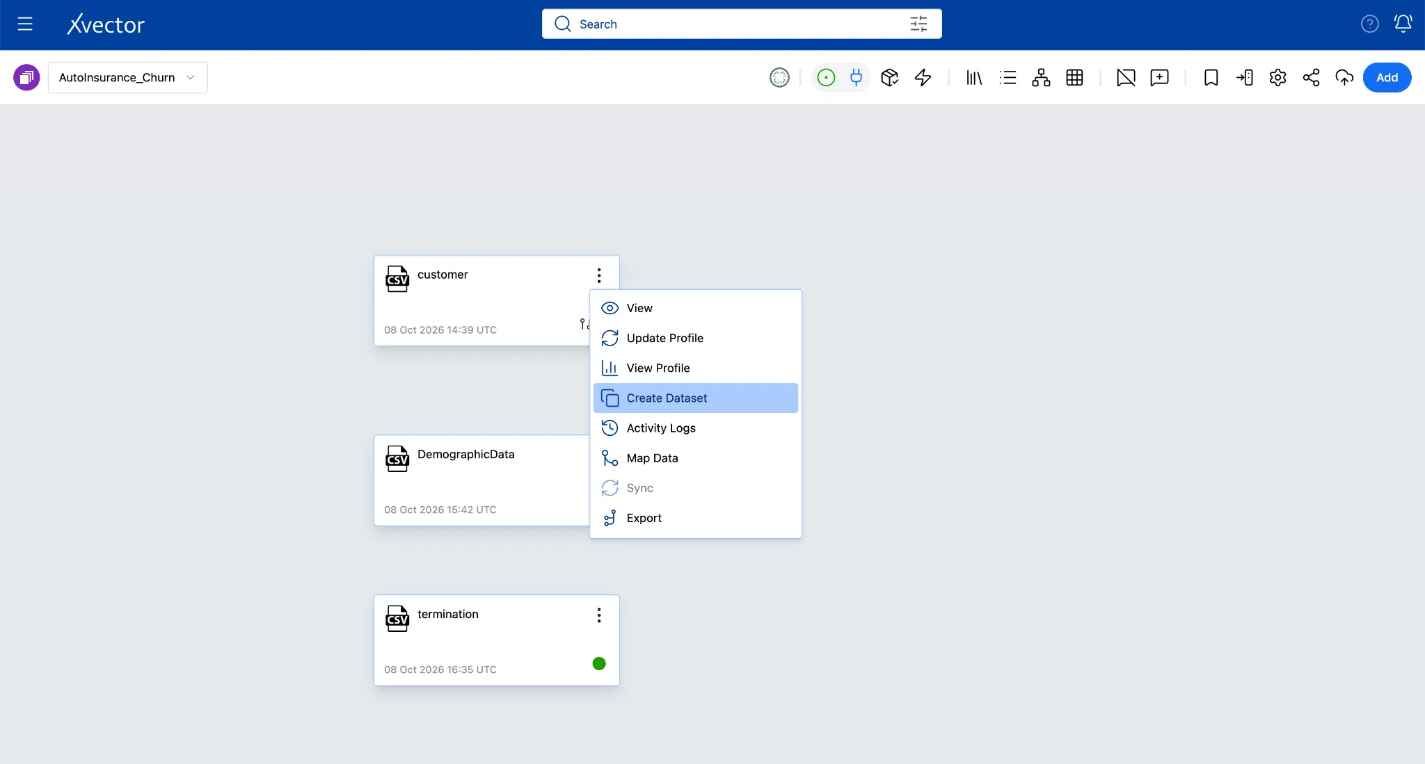
1. On the customer tile, click the ellipses (three dots) and choose Create Dataset.

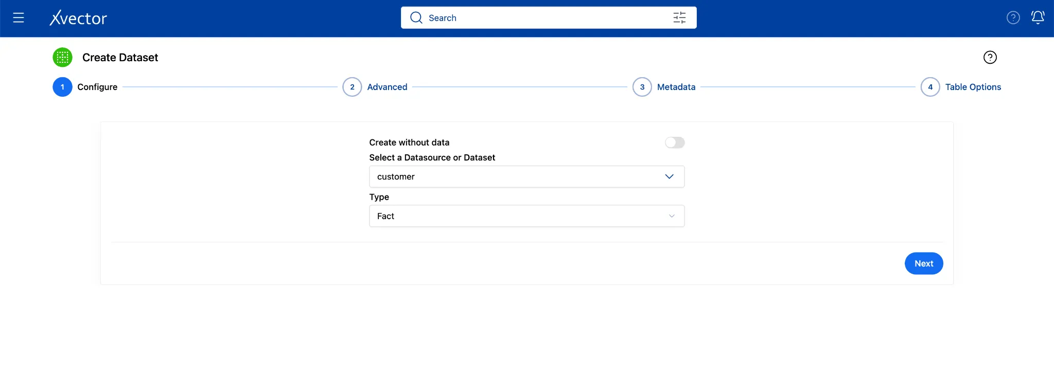
2. In the Configure step, select the Dataset from the dropdown as Customer

3. Type: Select Fact (default). This is a collection of insurance policy records, one row per policyholder event

4. Click Next

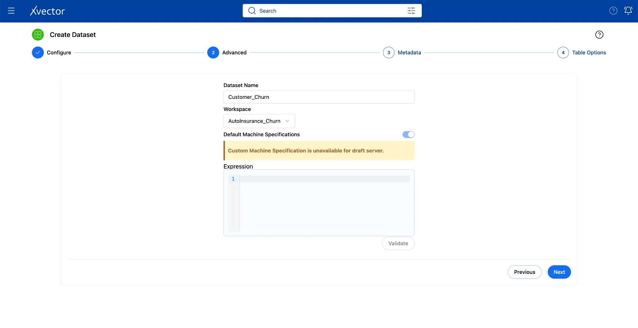
5. In the Advanced step, name it Customer_Churn and choose workspace: AutoInsurance_Churn**.**

6. Click Next

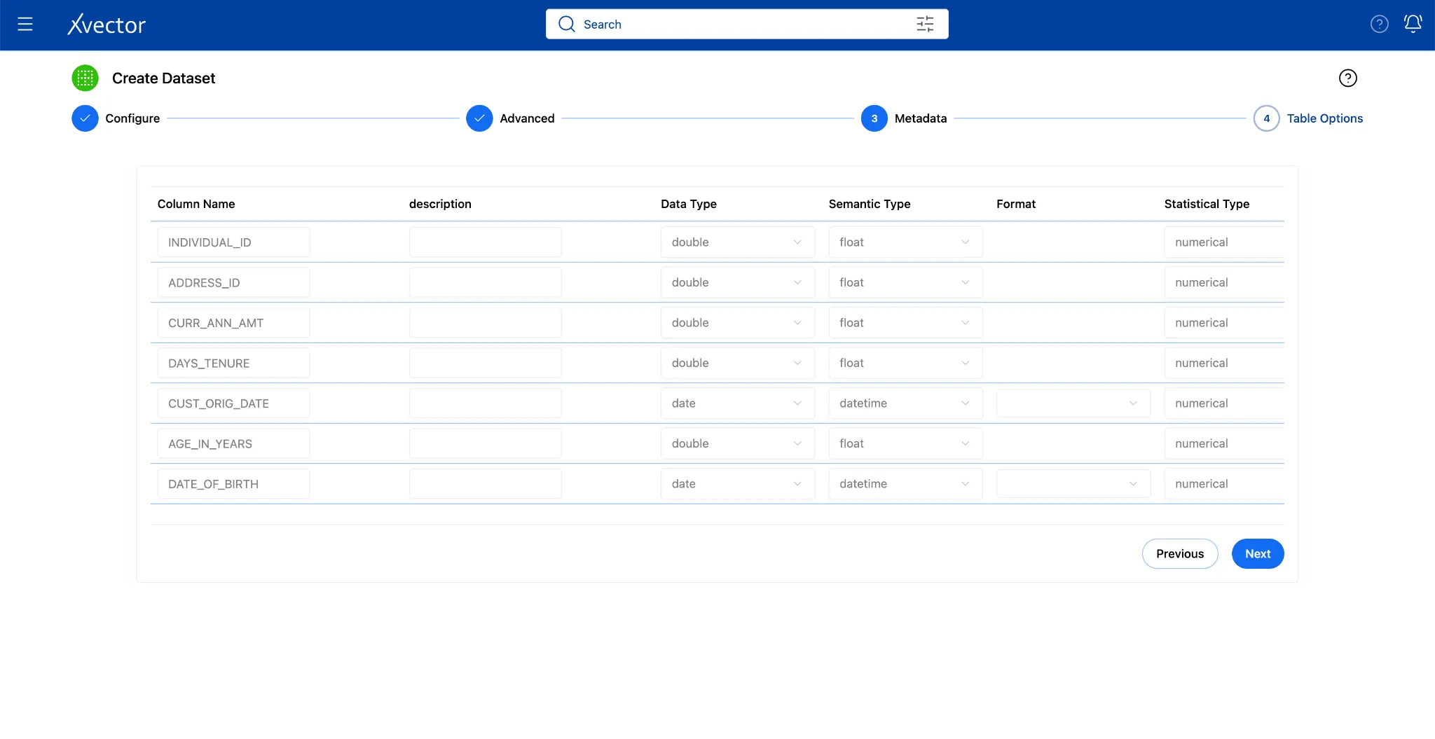
7. Leave the Table Options at their defaults. Click Create**.**

8. Click on Workspace once the “Successful” icon appears on the screen.

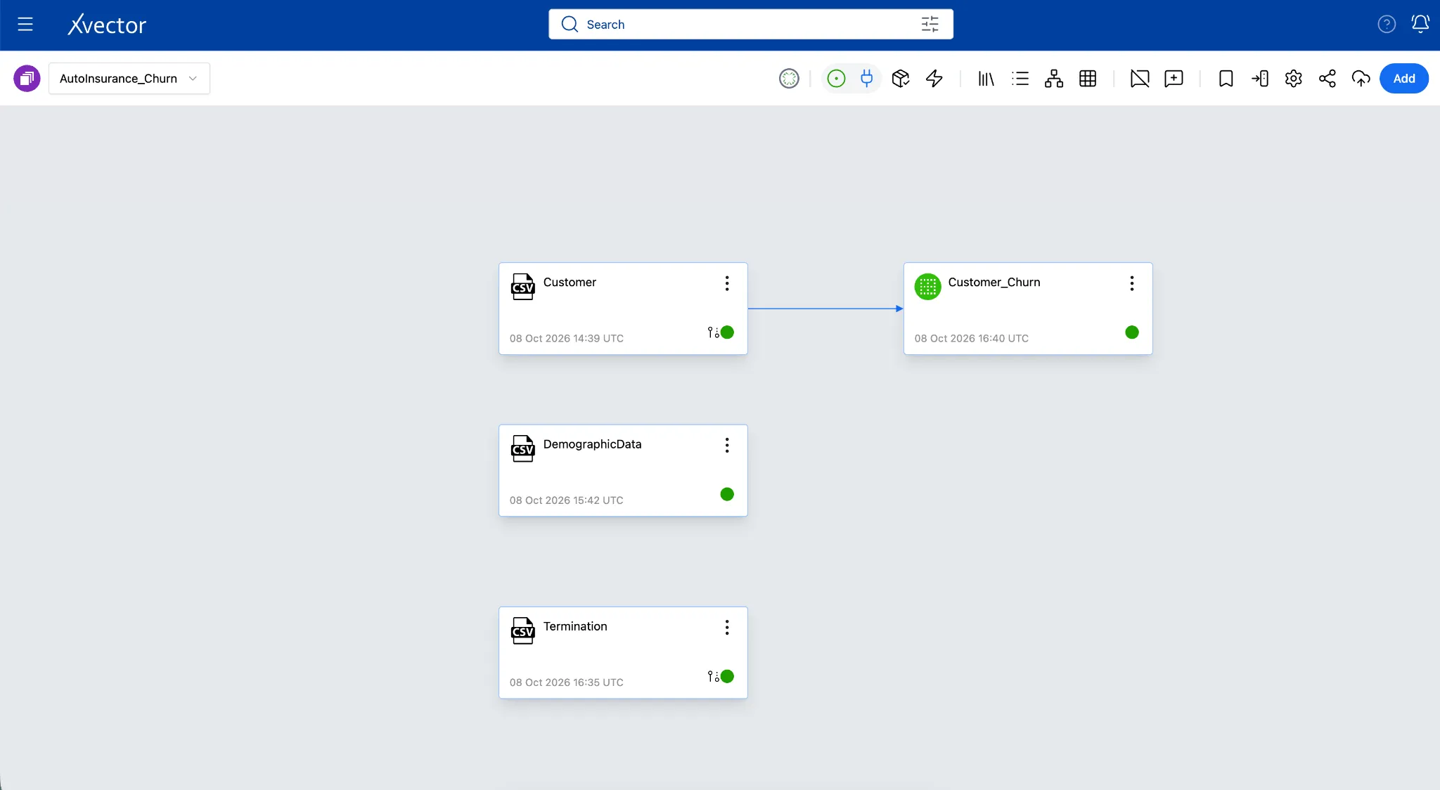
A Customer_Churn tile with a green dot appears. Double-click it to open the dataset view.

Step 4: Enrich Your Dataset

Raw data is rarely analysis-ready out of the box and often needs cleanup for missing values, placeholder rows, or unformatted columns. xVector solves this with enrichment functions that apply targeted transformations in the exact sequence you define, turning raw exports into clean, business-ready datasets. Here’s how we can implement them:

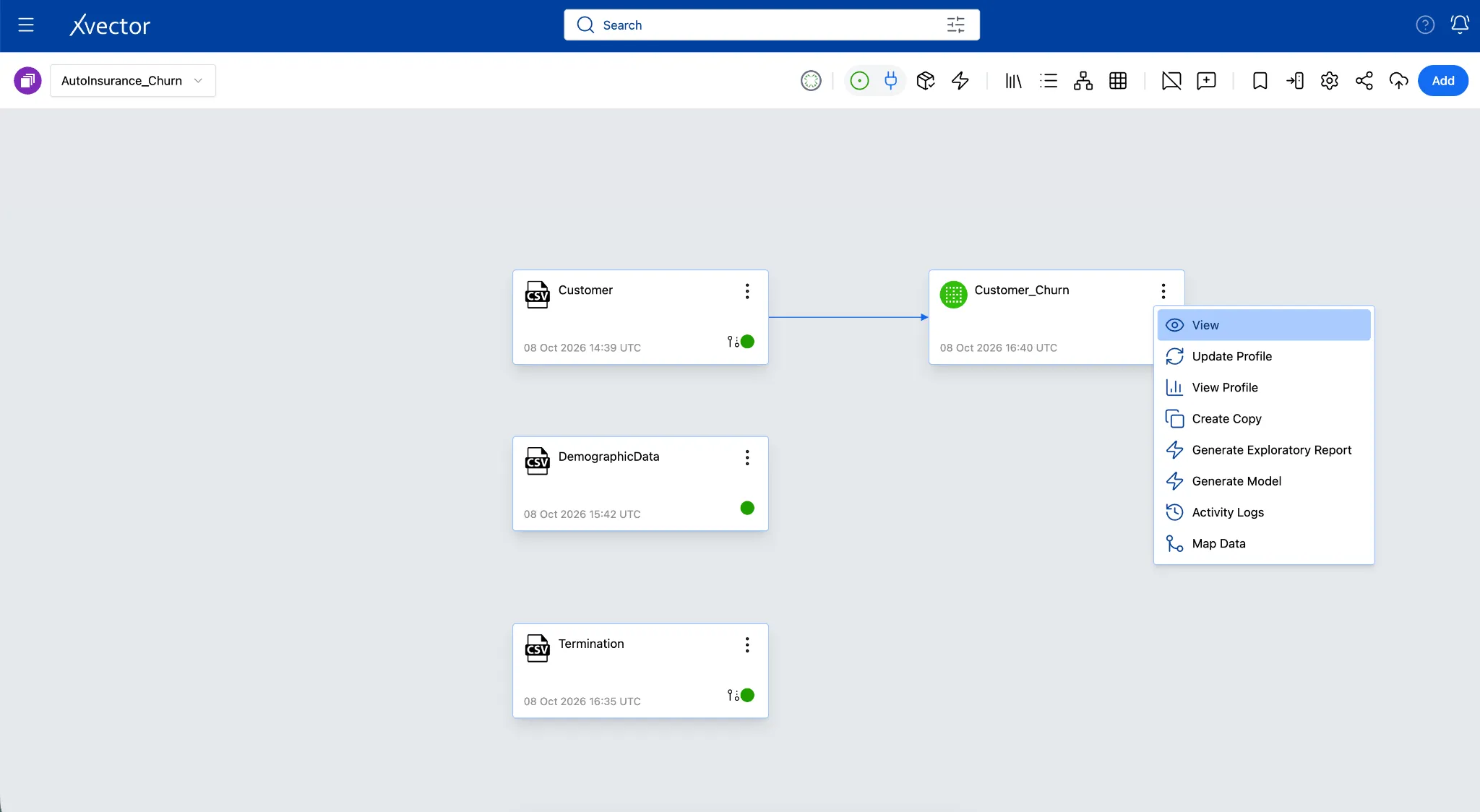
1. From the Workspace, locate the required Dataset tile.

2. Click the ellipses (three dots) on the Dataset and select View.
   OR double-click the Dataset tile to open the Dataset View.

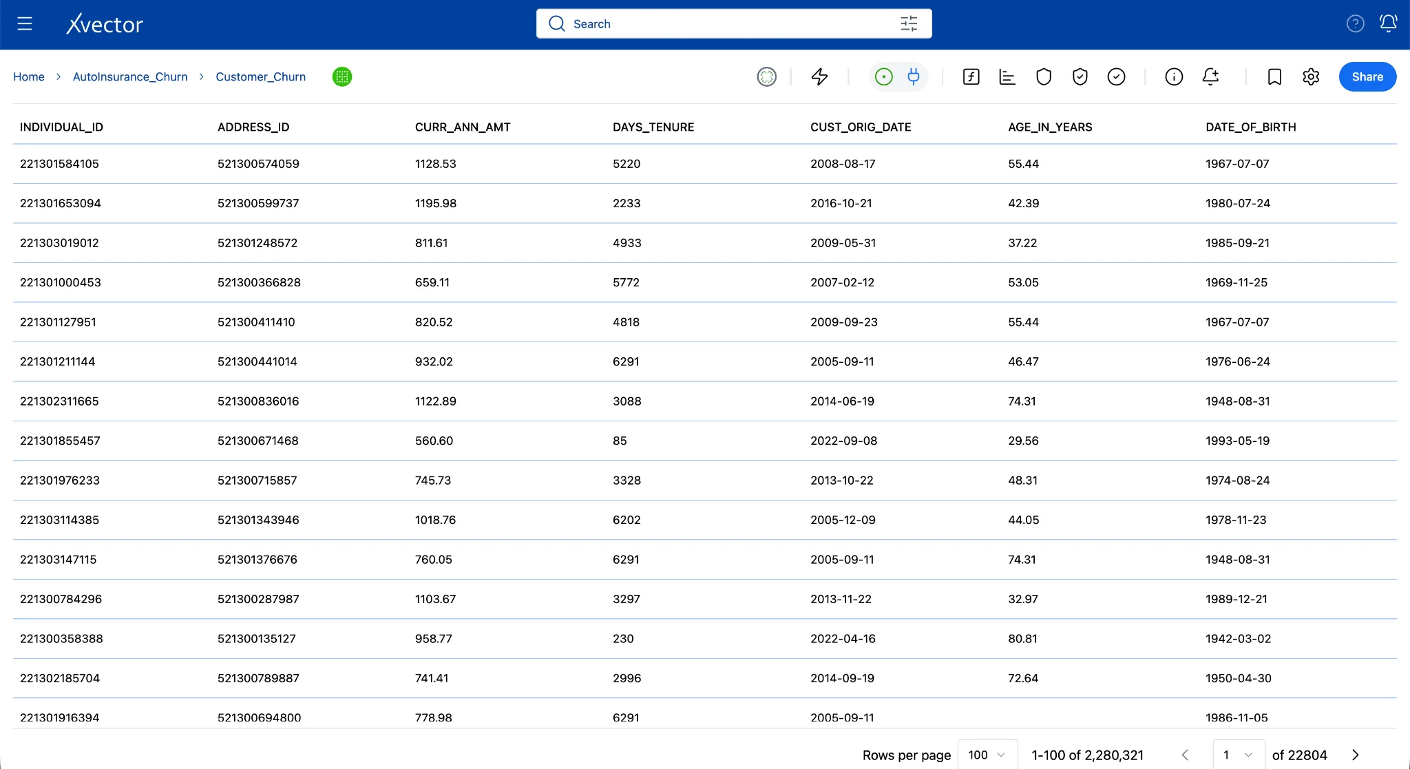
3. In the Dataset View, ensure the Draft Driver is running and the icon is green before performing enrichment.

4. Click the Data Enrichment (f) icon in the Dataset View toolbar.

5. In the XFlow Actions panel, click Add an action and choose the required enrichment function. You will add four functions in the order below; each builds on the previous one.

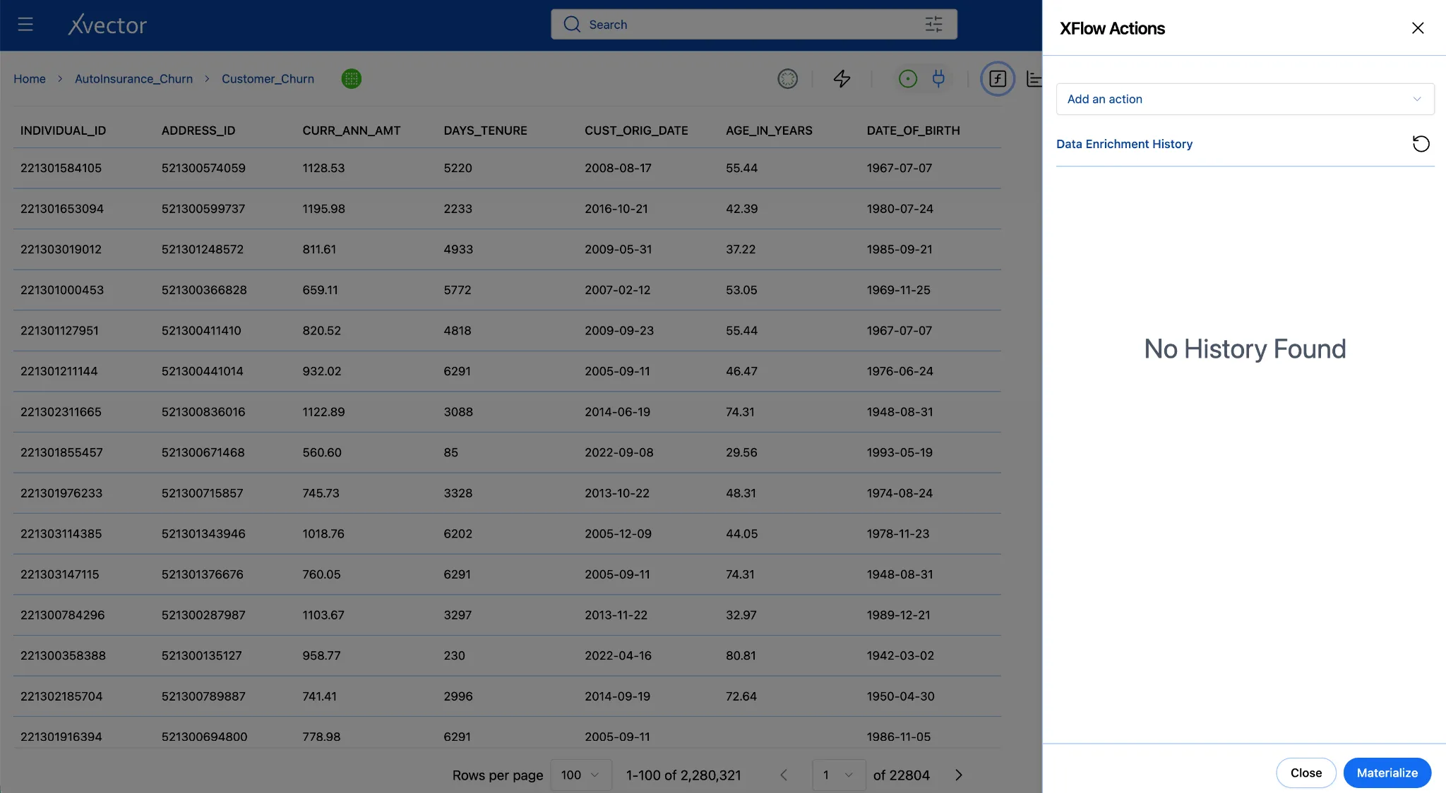
For every function: configure → Validate → Save. Do not skip Validate; it catches errors before they affect your data.

4a. Filter - Remove Invalid Records

The individual_id is the unique identifier for every policyholder; it is also the key you will use to join demographics. Records with an ID of 0 or below are system placeholders or data-entry errors that have no corresponding demographic record and no business meaning. Removing them first ensures every downstream step operates only on real policyholders and the join isn’t skewed by unmatched placeholder rows.

1. Click Add an action and select Filter.

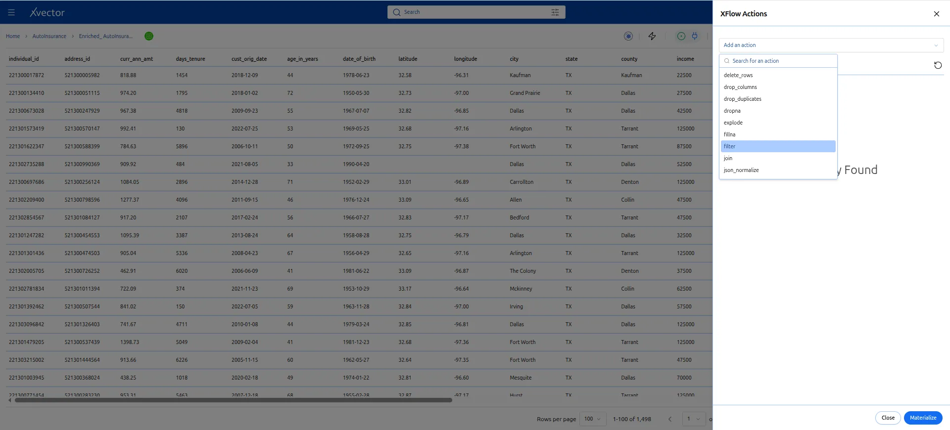
2. Enter the expression: Select * from dataset where individual_id > 0;

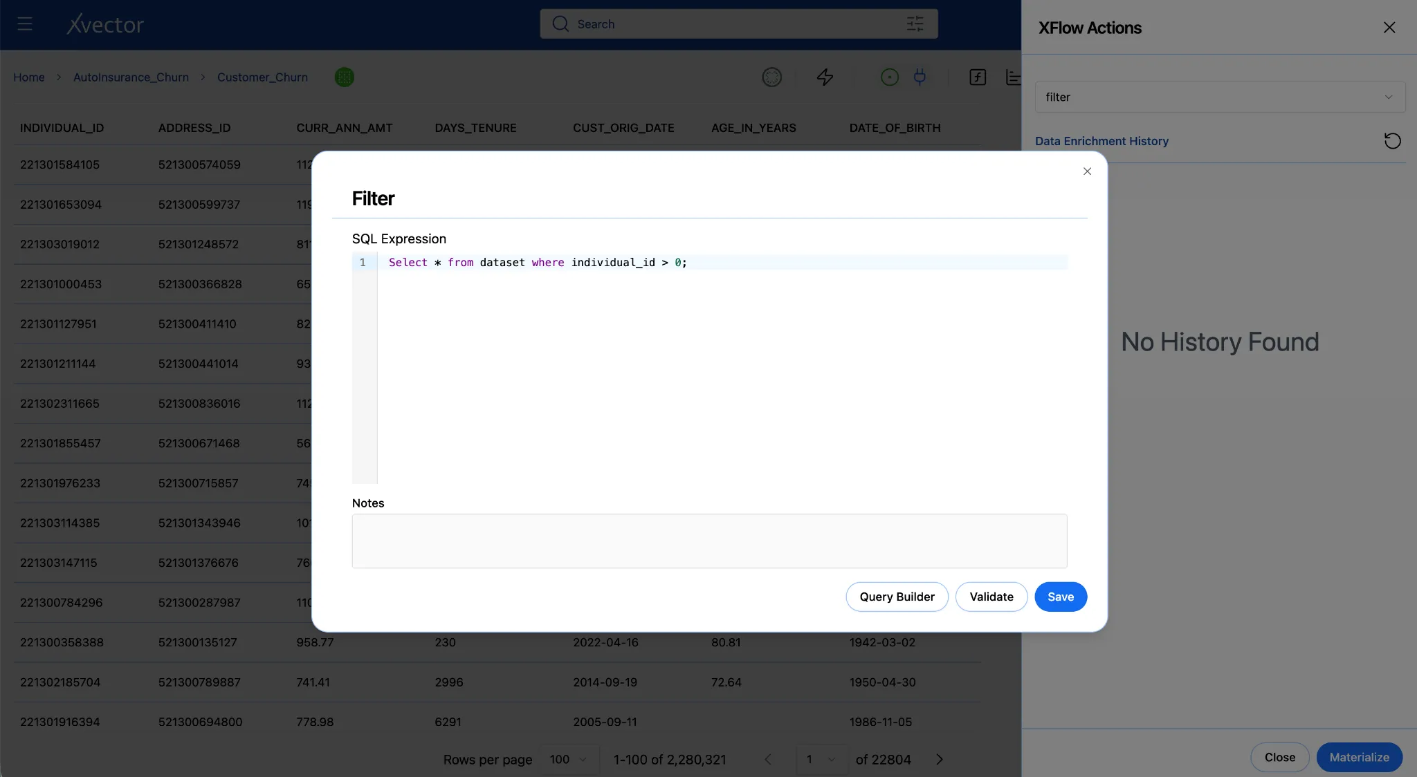
3. Click Validate. You should see a confirmation with a record count.

4. Click Save.

What to expect

The record count in your dataset view may drop slightly after the filter.

If it drops by more than a few percent, pause and investigate; there may be a data quality issue worth flagging before you go further.

4b. Fillna - Handle Missing Ages

After removing invalid records, address data completeness. A small number of policyholders may have a null age_in_years, typically because age was not captured at enrollment or was redacted. Null values in a numeric column produce misleading averages in charts that exclude part of the population and can break certain visualizations entirely. Replacing them with a reasonable default keeps the dataset complete without dropping rows that have valid churn data.

1. Click Add an action and select Fillna.

2. Configure with the following values:

Field	Value
Column	age_in_years
Fill Value	45
Fill Method	Mean

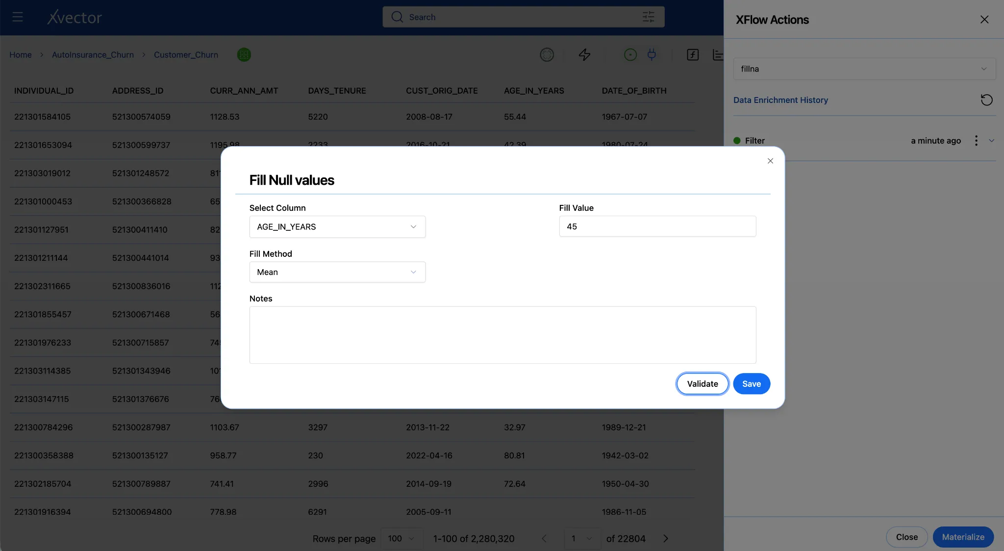
3. Click Validate, then Save.

Where does 45 come from?

The sample data shows most policyholders are in their 40s and 50s. 45 is domain-reasonable and avoids distorting the age distribution. For a production dataset, run a Profile on the datasource first (ellipses on the datasource tile → Update Profile → View Profile) to find the actual median, then use that value instead.

4c. Join - Merge Demographics and termination into Your Dataset

For now, assume we have clean, complete insurance records. To understand why customers churn, you need to know who they are: their income, education, household composition, and financial standing. The JOIN function connects Customer_Churn to the DemographicData datasource on the shared individual_id, adding those demographic columns to every matching policyholder row.

A LEFT JOIN keeps every row from Customer_Churn and adds matching columns from DemographicData where individual_id matches. Policyholders with no demographics match keep their row; the added columns will be null.

Since we are not modifying the individual_demographics datasource, we can join this datasource directly into the Customer_Churn dataset. We don’t need to create a dataset for DemographicData and then join it.

1. Click Add an action and select Join.

2. Configure:

Field	Value
Join Type	Left
Target Dataset	DemographicData
Left key (customer_churn)	individual_id
Right key (demographics)	INDIVIDUAL_ID

3. In the Expression pane, delete everything that is given

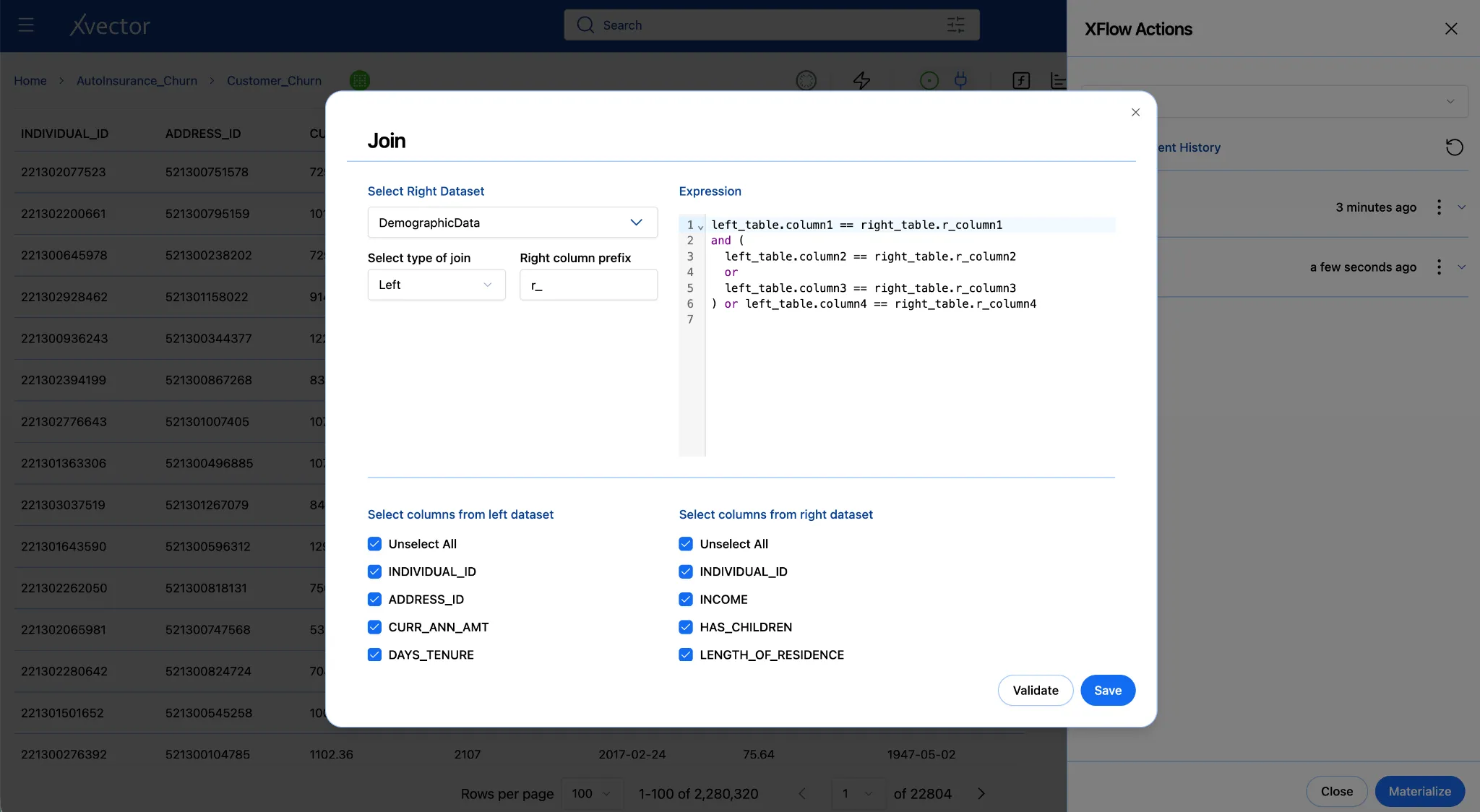
4. Add the expression in the Expressions pane:

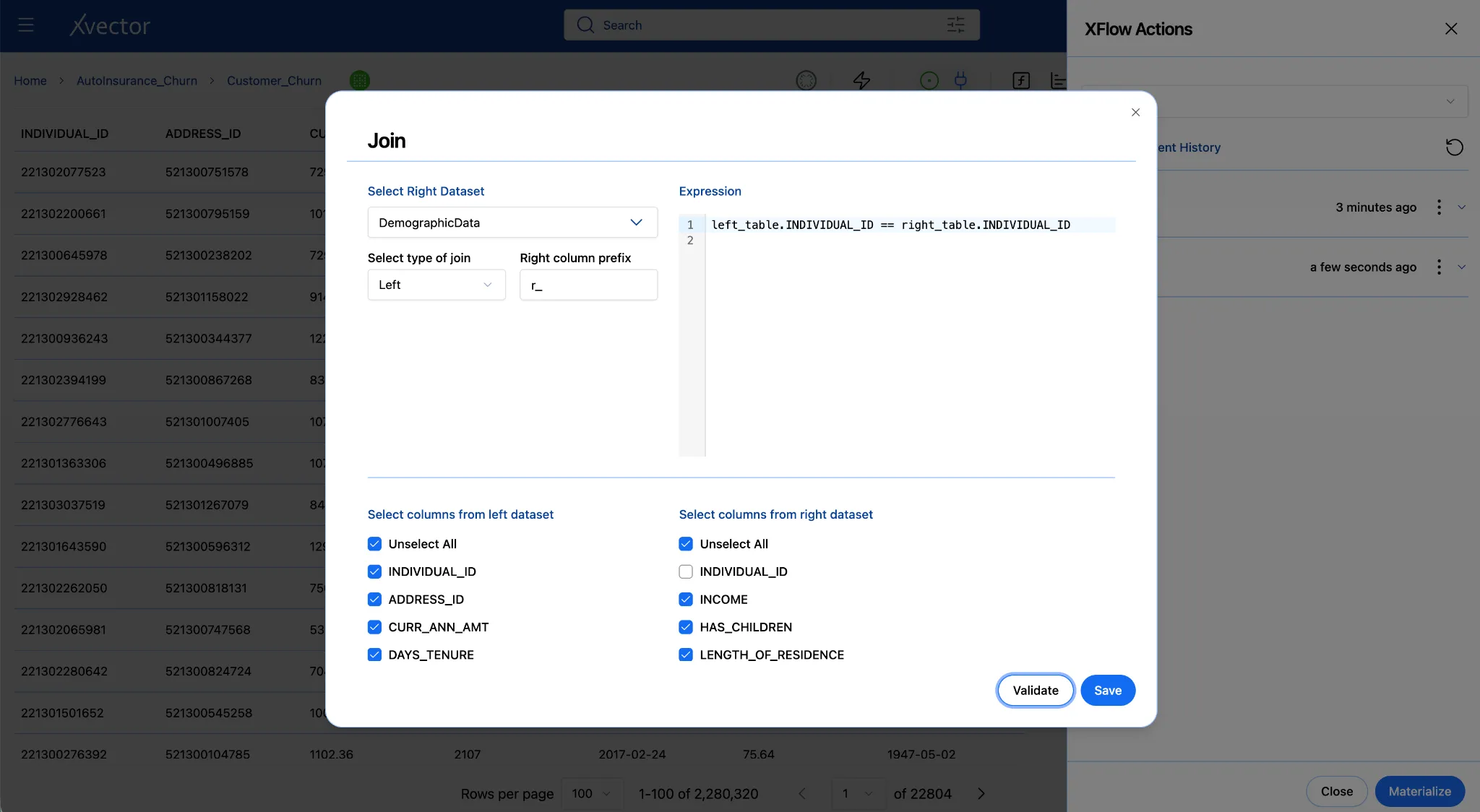
“left_table.individual_id == right_table.INDIVIDUAL_ID”

5. Since individual_id is the primary key and will be the same in both datasets, we can uncheck INDIVIDUAL_ID from the right dataset.

6. Click Validate.

7. Click Update.

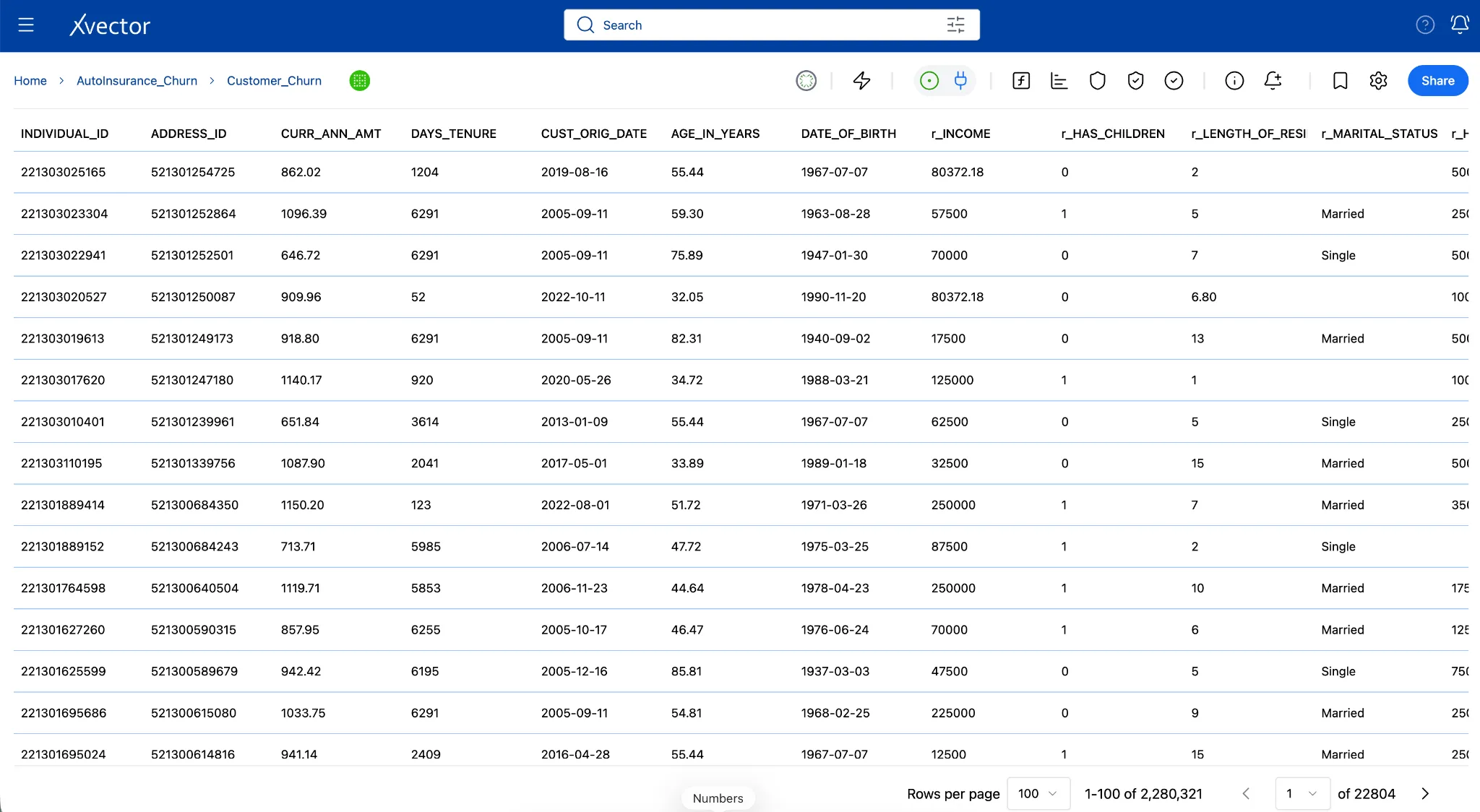
All the new columns in the dataset will now show columns that start with r_.

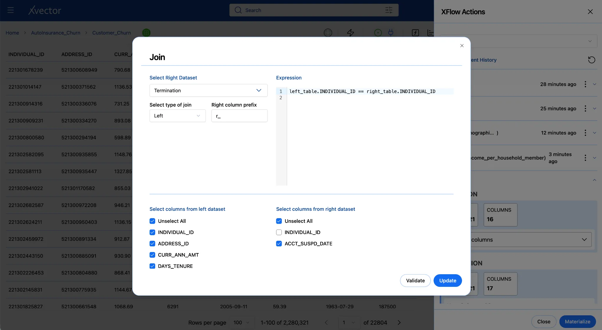
Join - Termination dataset

Join the termination dataset with the Customer_Churn dataset to bring in the ACCT_SUSPD_DATE for customers. This will eventually let us derive a flag indicating whether a customer has churned.

Note: This was done after New Column in the example here, but it can be done before as well.

Note the column names before moving on

After the join, open the dataset column list and note how xVector named the incoming income column. It may appear as r_INCOME since the right-hand column prefix we chose above is “r_”.

4d. New Column - Income per Household Member and Churn

Income Per Household Member

The join has given you both income and household composition data for each policyholder. Now use them together. A policyholder’s raw income isn’t a fair indicator of financial strain on its own; $40,000 means something very different for a single person than for a married couple with children. Dividing income by estimated household size creates a normalized measure of per-person financial capacity. A customer who is financially stretched relative to their household is more likely to cancel a non-essential cost like auto insurance than one with the same income and no dependents.

Household size logic:

Situation	Estimated household size
Has children	3 (couple + kid, conservative estimate)
Married, no children	2
Single, no children	1

1. Click Add an action and select New Column.

2. Configure:

Field	Value
New Column Name	income_per_household_member
Data Type	float

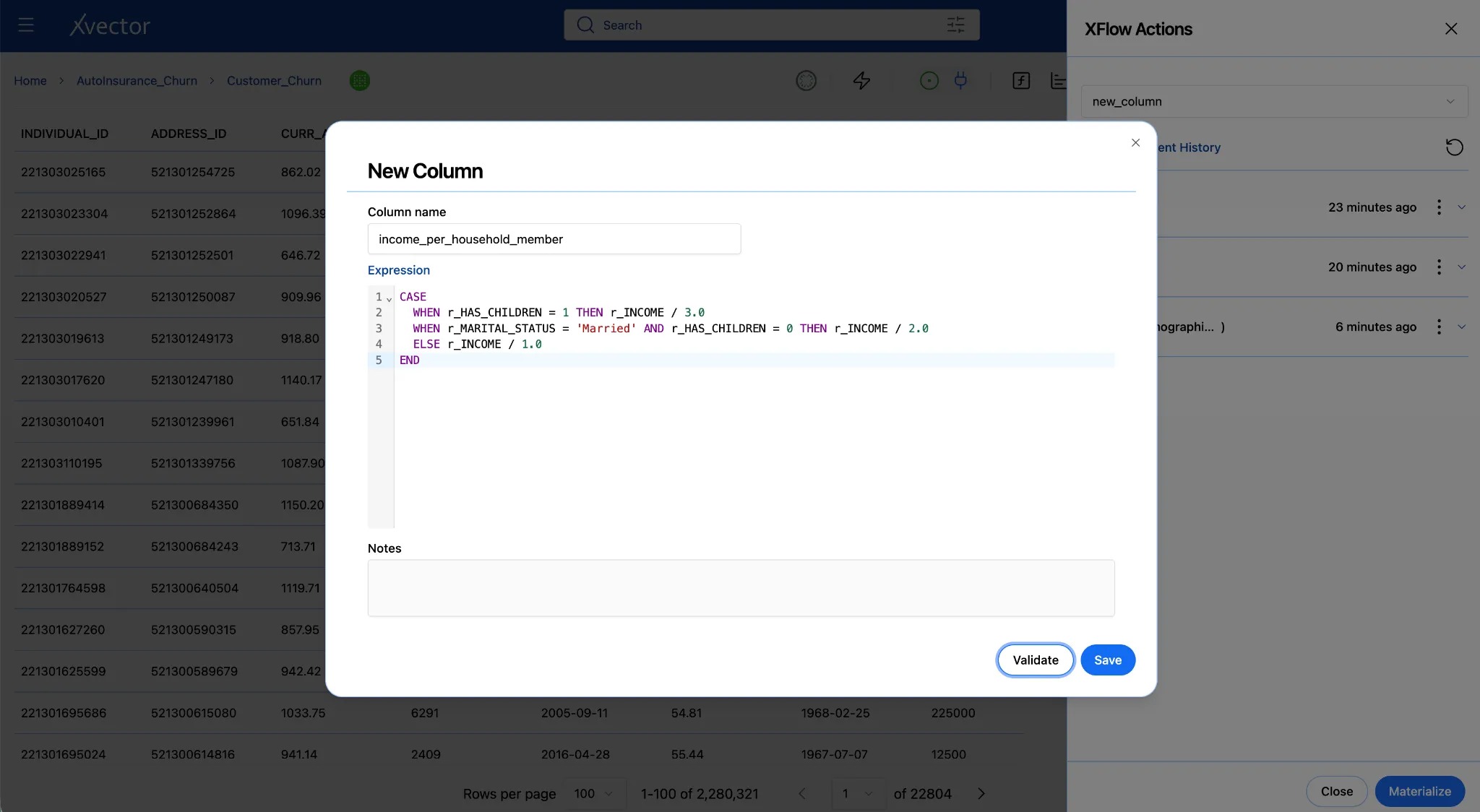
3. Enter the expression below. Adjust the column name income to match exactly what you saw in Step 4c:

CASE
WHEN r_HAS_CHILDREN = 1 THEN r_INCOME / 3.0
WHEN r_MARITAL_STATUS = 'Married' AND r_HAS_CHILDREN = 0 THEN r_INCOME / 2.0
ELSE r_INCOME / 1.0
END

Column name variants after the join

The new columns that we brought in via the join have r_ as a prefix. Please use these prefixed columns to create the New Column, “income_per_household_member”.

4. Click Validate.

5. Click Save. You can see the new column gets created at the end of the dataset.

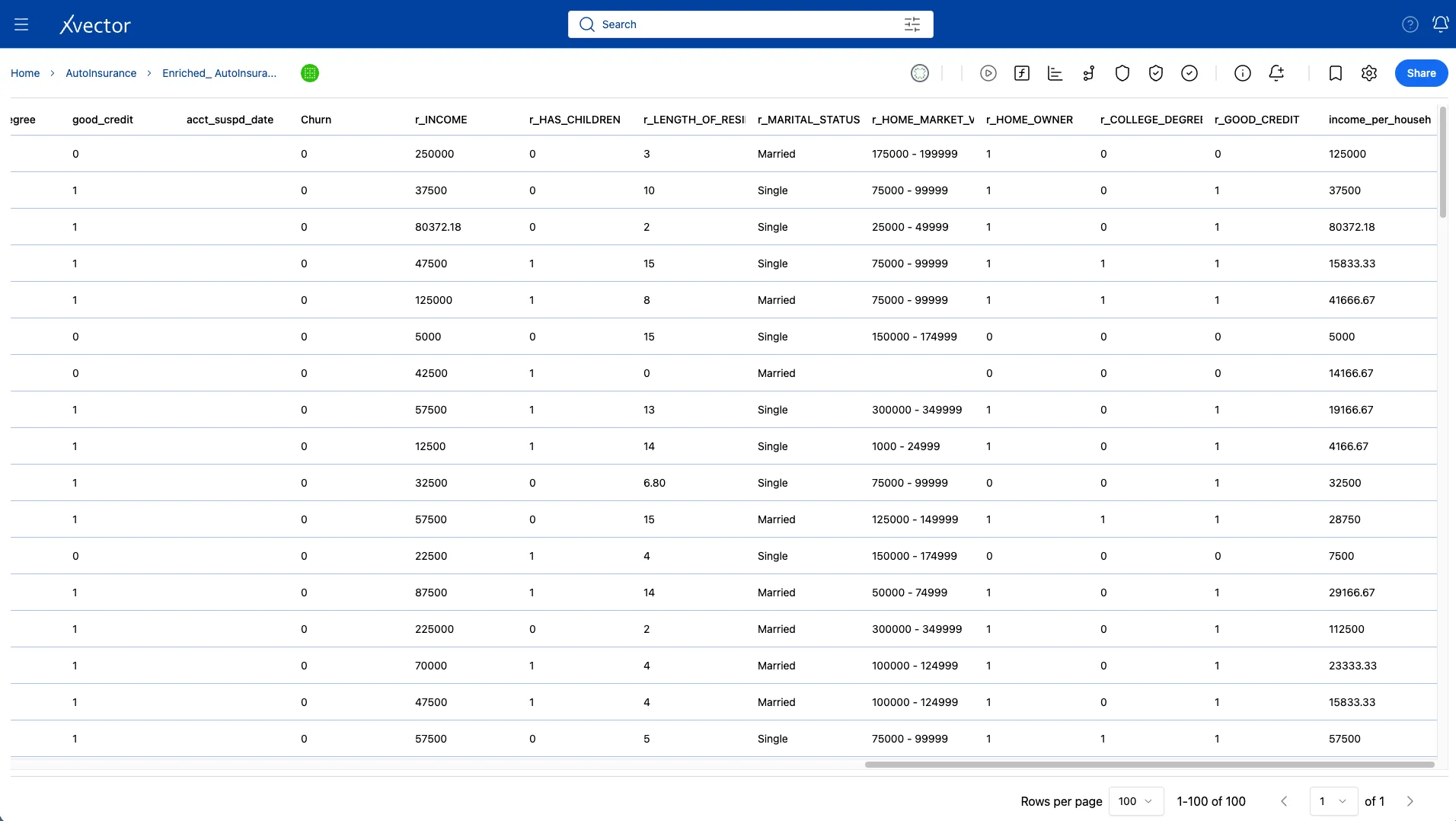
New Column - churn

Joining the Customer_Churn dataset with the Termination dataset brings in the suspended/cancelled date for customers. We can now create a new column called churn, where the value is 1 if ACCT_SUSPD_DATE has a value. If the value is blank, then the customer has not churned, and the value is 0.

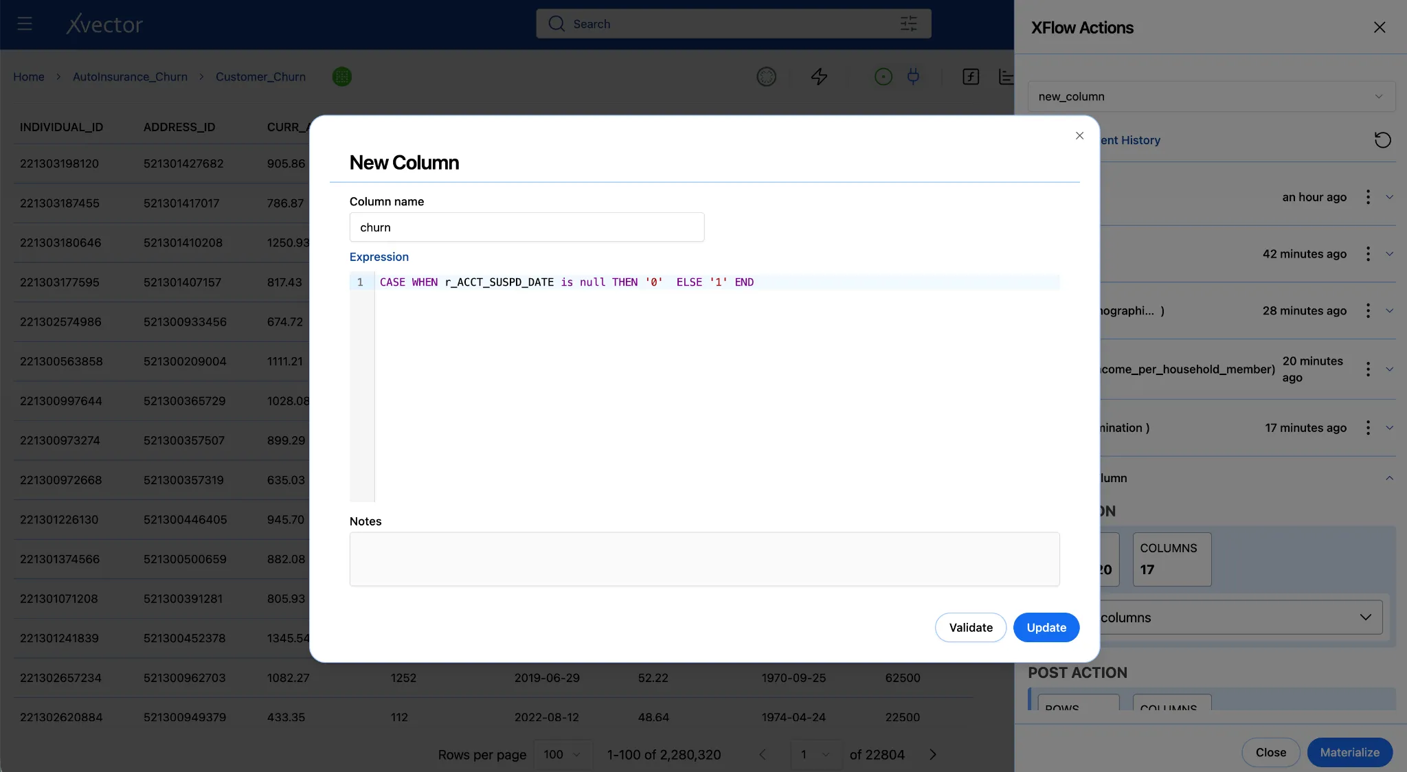
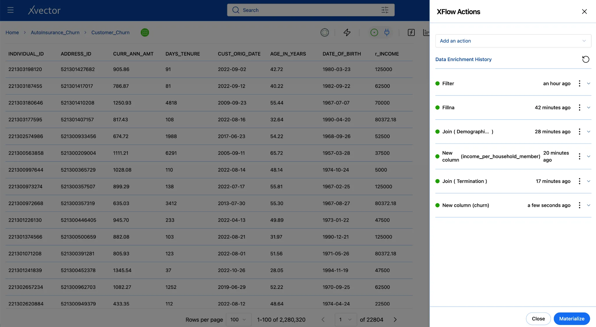
4e. Materialize - Write the Enriched Data to Storage

Saving enrichment functions records their logic, but it doesn’t persist the dataset. Since we are working with the draft driver, the enriched dataset is only in memory. Materializing runs all four functions in sequence and writes the final enriched dataset to storage, making it available for reporting and modeling. Materialize persists the enriched data.

1. In the enrichment panel, scroll to the bottom.

2. Click Materialize (Leave the default options)

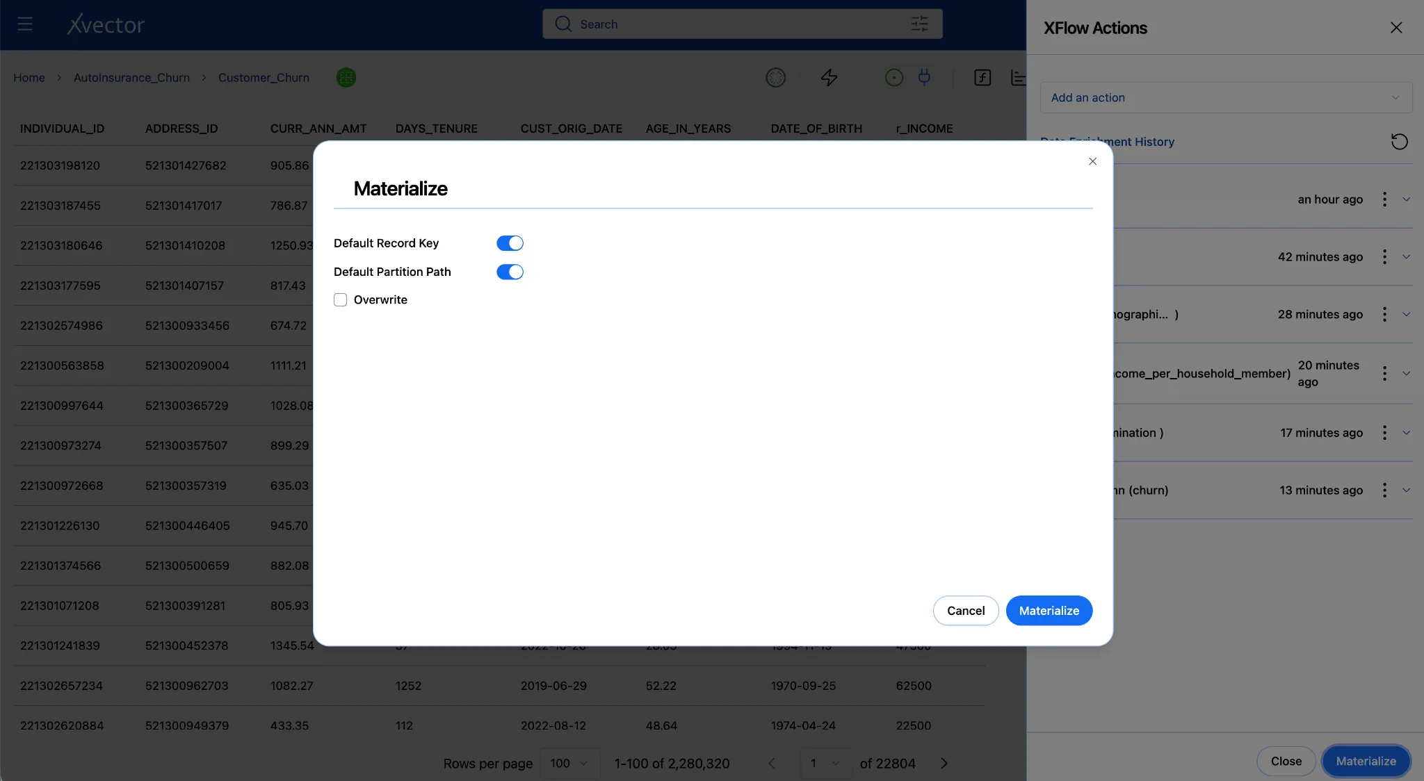
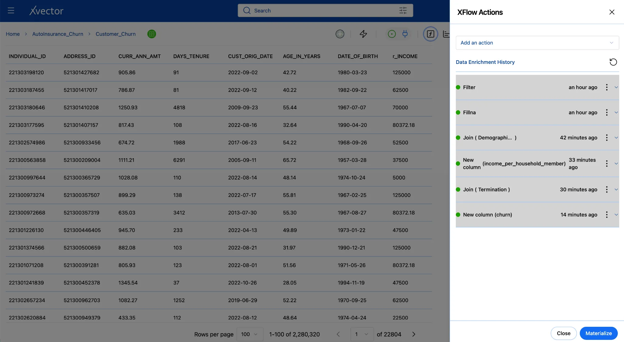
3. After clicking Materialize, the enriched dataset is displayed with the applied transformations and newly added columns

Troubleshooting Enrichment

Problem	Most likely cause	Fix
The enrichment panel does not respond	Draft driver not running	Click the play button (▶) in the toolbar in the workspace; wait for the icon to turn green
Join returns zero new columns	Key column name mismatch	Verify both sides use the individual_id
The chart shows blank or no data	Report driver not running	Click the play button (▶) in the toolbar in the workspace; wait for the icon to turn green

Step 5: Build the Dashboard

With an enriched, materialized dataset, you can now turn the data into a story. Reports in xVector are live, interactive dashboards, not static exports. Each component on a report sheet pulls directly from a dataset, so charts update when the underlying data changes. Users can apply filters, drill into details, and leave comments without touching the dataset itself.

You will build a report with three sheets, each answering a churn question. The report will help you understand the churn profile by marital status, breakdown by credit quality, and who the high-value customers are to prioritize for retention.

1. From the workspace, click Add and select Report.

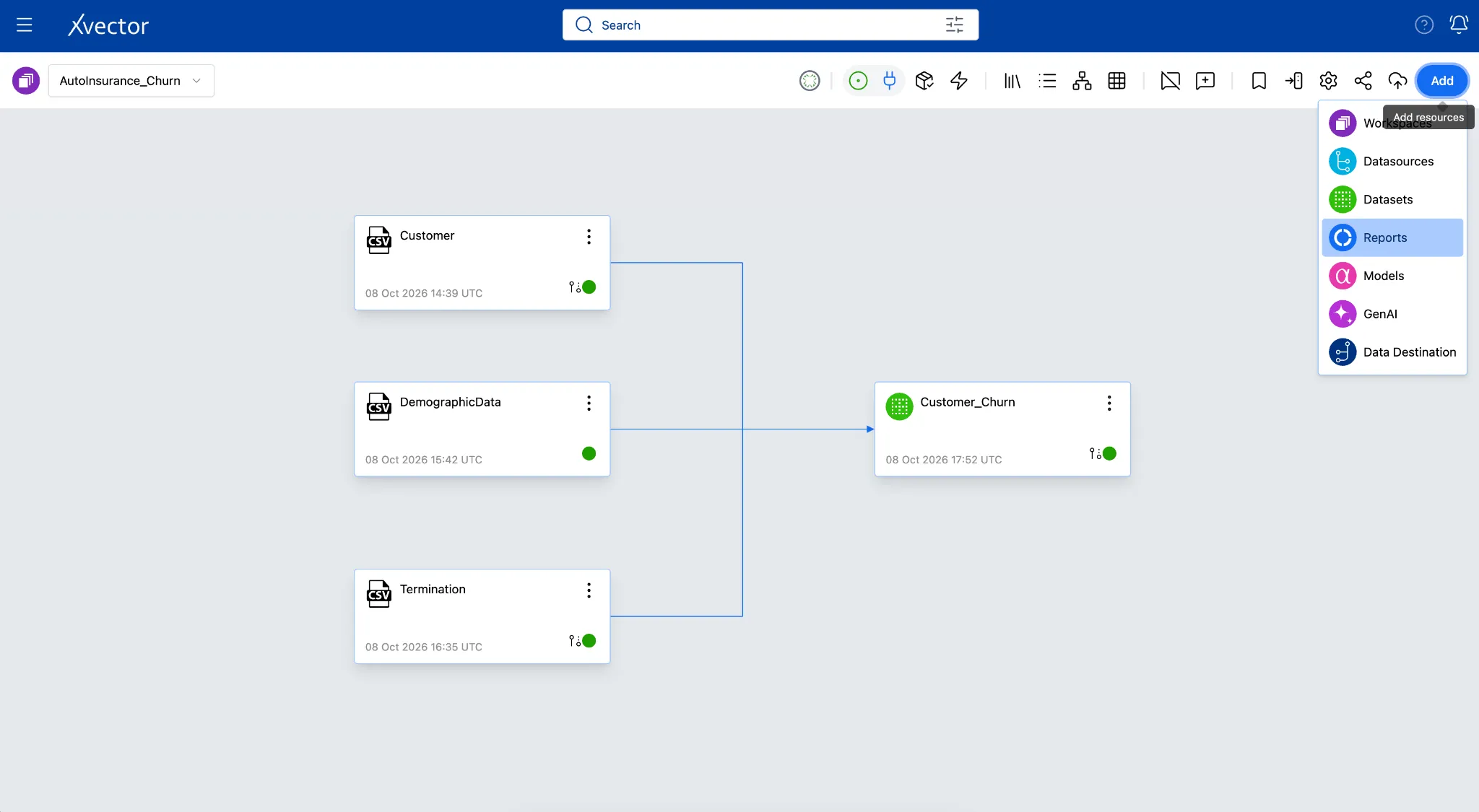
2. Rename the “untitled report” (top-left breadcrumbs) by double-clicking it on the Report page to “AutoInsurance_Churn_Dashboard”

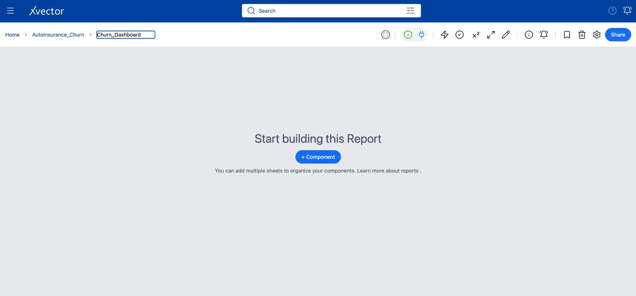
3. Ensure the Draft Driver is on.

Sheet 1 - Churn Profile by Marital Status (Bar Chart)

Business question: Are certain demographic profiles significantly more likely to churn?

Understanding whether churn concentrates in specific marital status segments helps retention teams target their outreach. A married couple paying a high combined premium under financial strain behaves very differently from a single policyholder with the same raw income. This bar chart surfaces those contrasts at a glance by showing average annual premium across marital status groups, split by churn status.

A grouped bar chart with marital status on the X-axis, average annual premium on the Y-axis, and churn status as the color split gives an immediate view of which segments are most at risk.

Click the Pen icon to switch to Edit mode or click on. At the bottom of the report, locate Sheet-1, double-click the sheet name, and rename it Churn Profile.

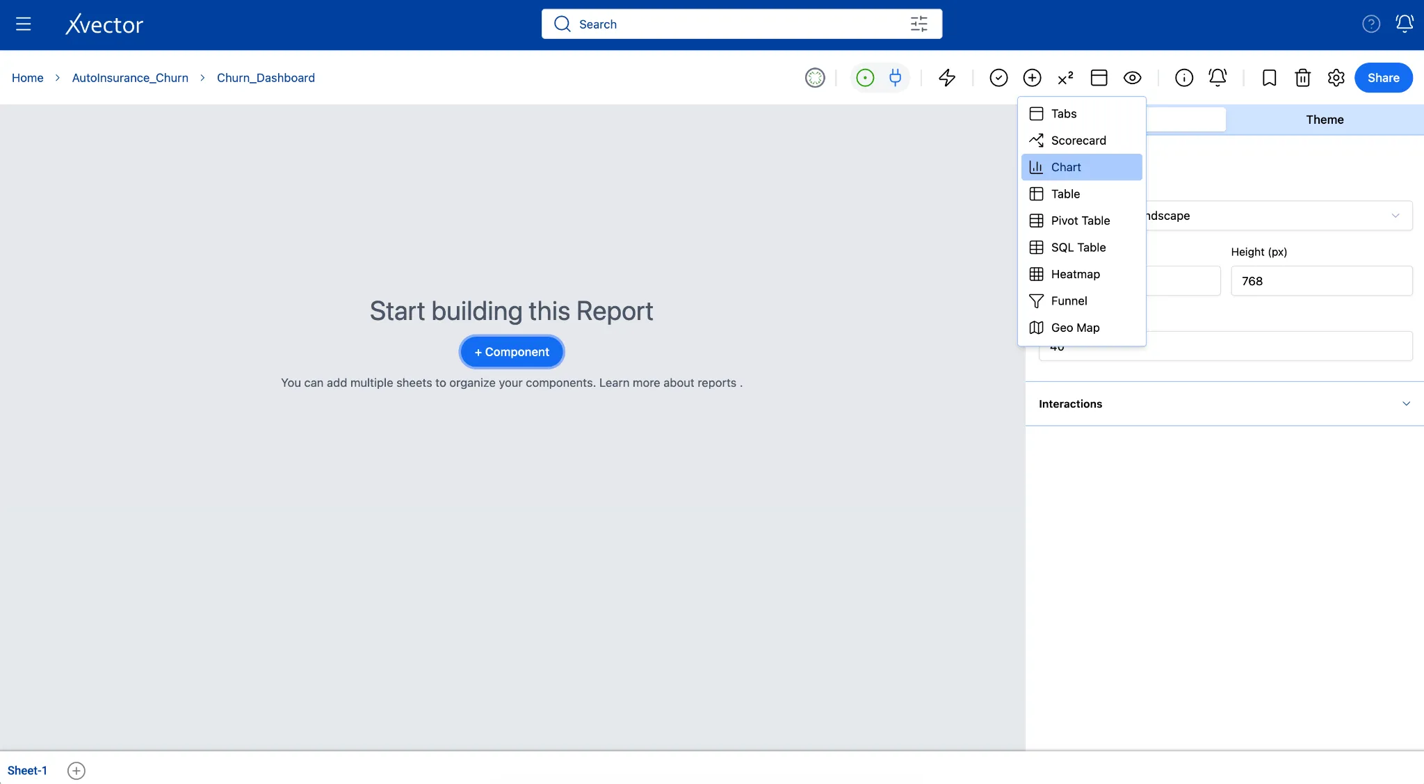
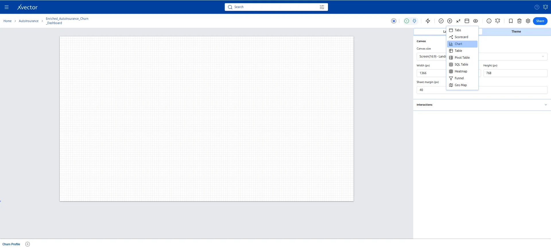
1. Click Add Component (+) and select Chart, Bar Chart.

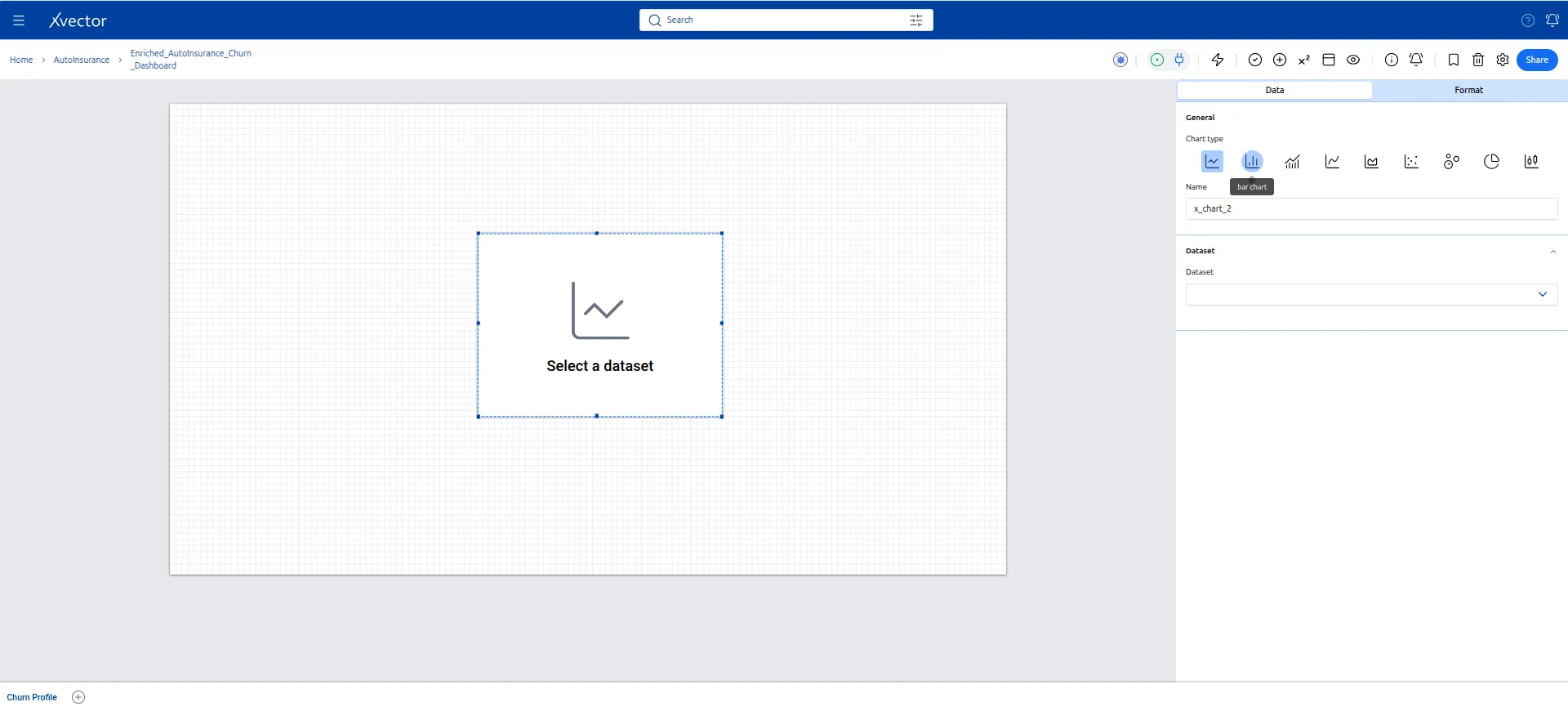
2. In the Data tab, add the following field values:

Setting	Value
Dataset	Customer_Churn
X-Axis (Dimension)	r_MARITAL_STATUS
Second Dimension	churn
Y-Axis (Measure)	curr_ann_amt with aggregate AVG
Sort	Descending by Y-axis

In the Format tab: set the title to Average Premium by Marital Status and Churn Status.

3. Resize to fill the sheet comfortably.

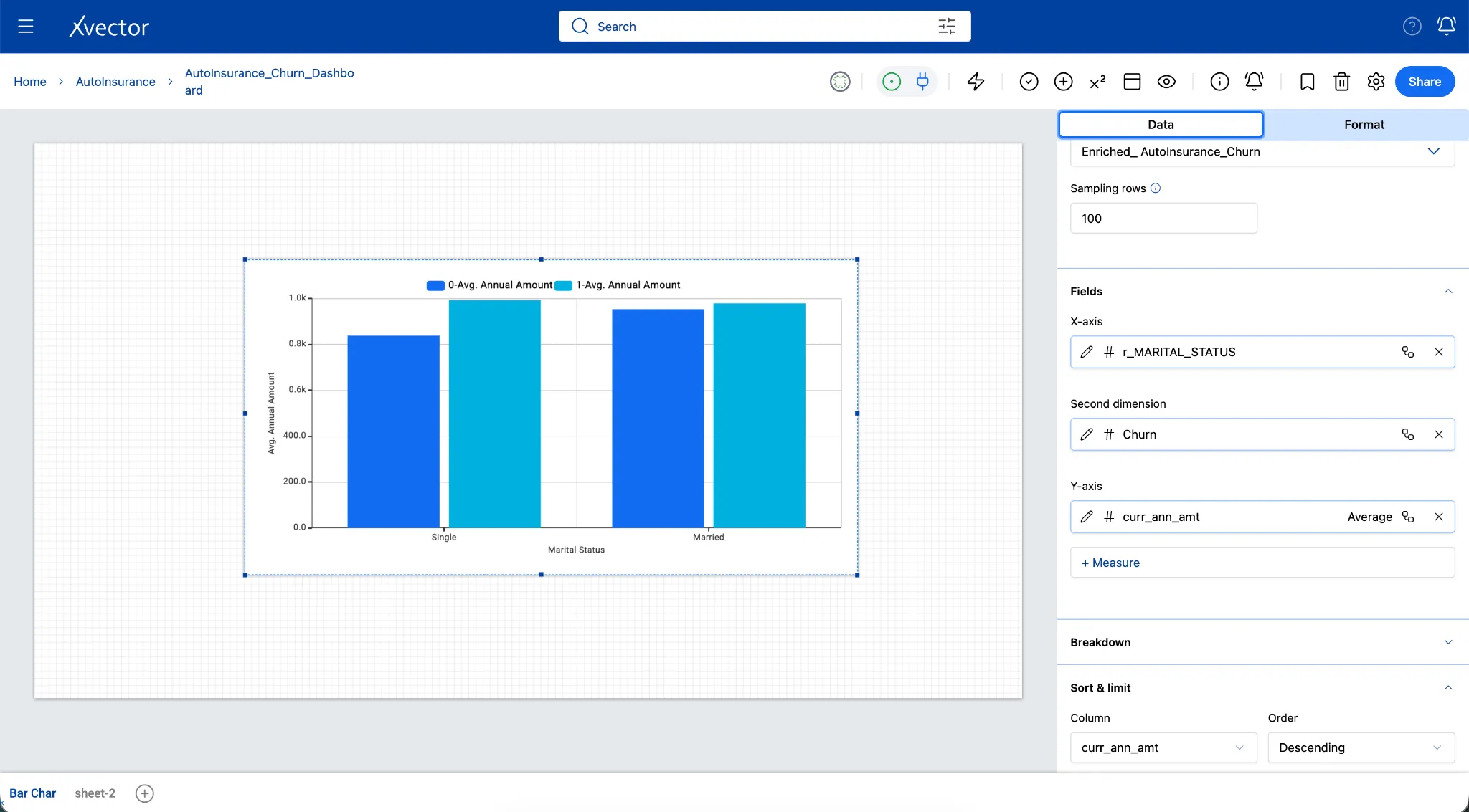
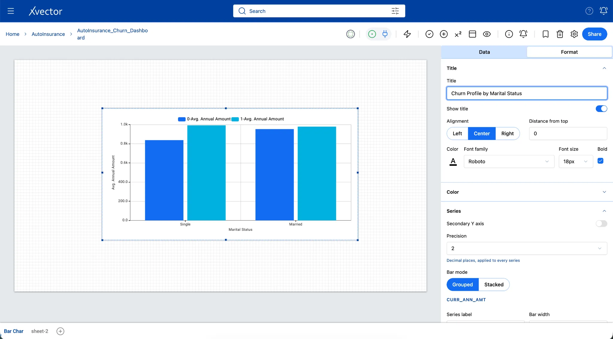
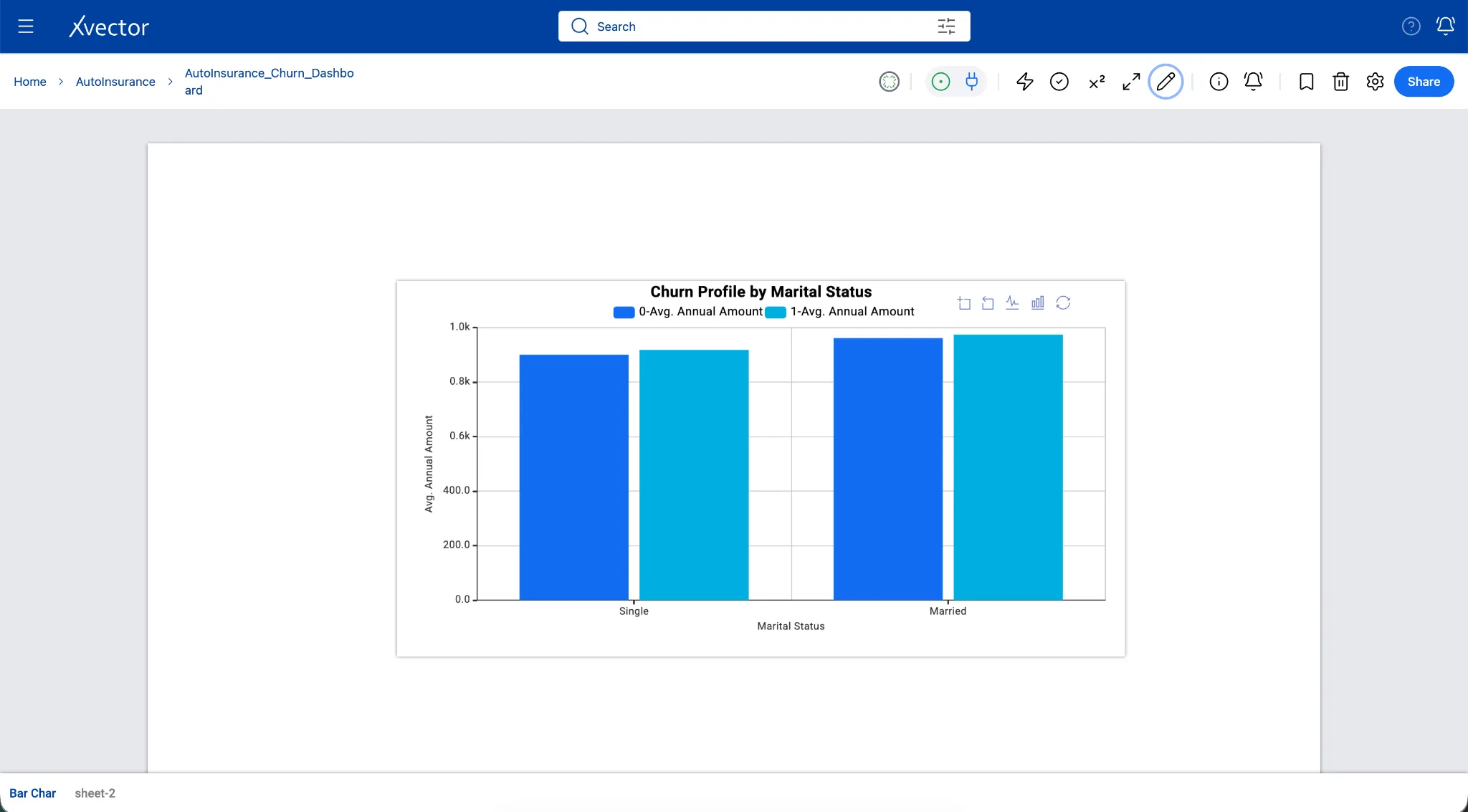
Note: If married policyholders paying higher premiums are churning at a higher rate than single ones, it suggests price sensitivity in the household. In the current scenario, the minimal variance between retained and churned averages suggests that premium is not a dramatic standalone driver of churn; retention teams should look beyond raw price points to engagement metrics, tenure, or claims history.

Sheet 2 - Breakdown by Credit Quality (Pie Charts)

Business question: Are customers with lower credit scores significantly more likely to cancel their auto insurance policies compared to those with good credit?

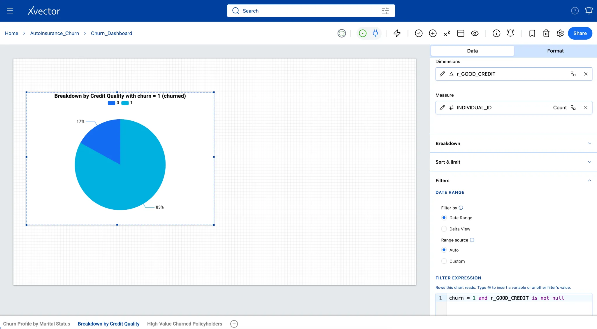
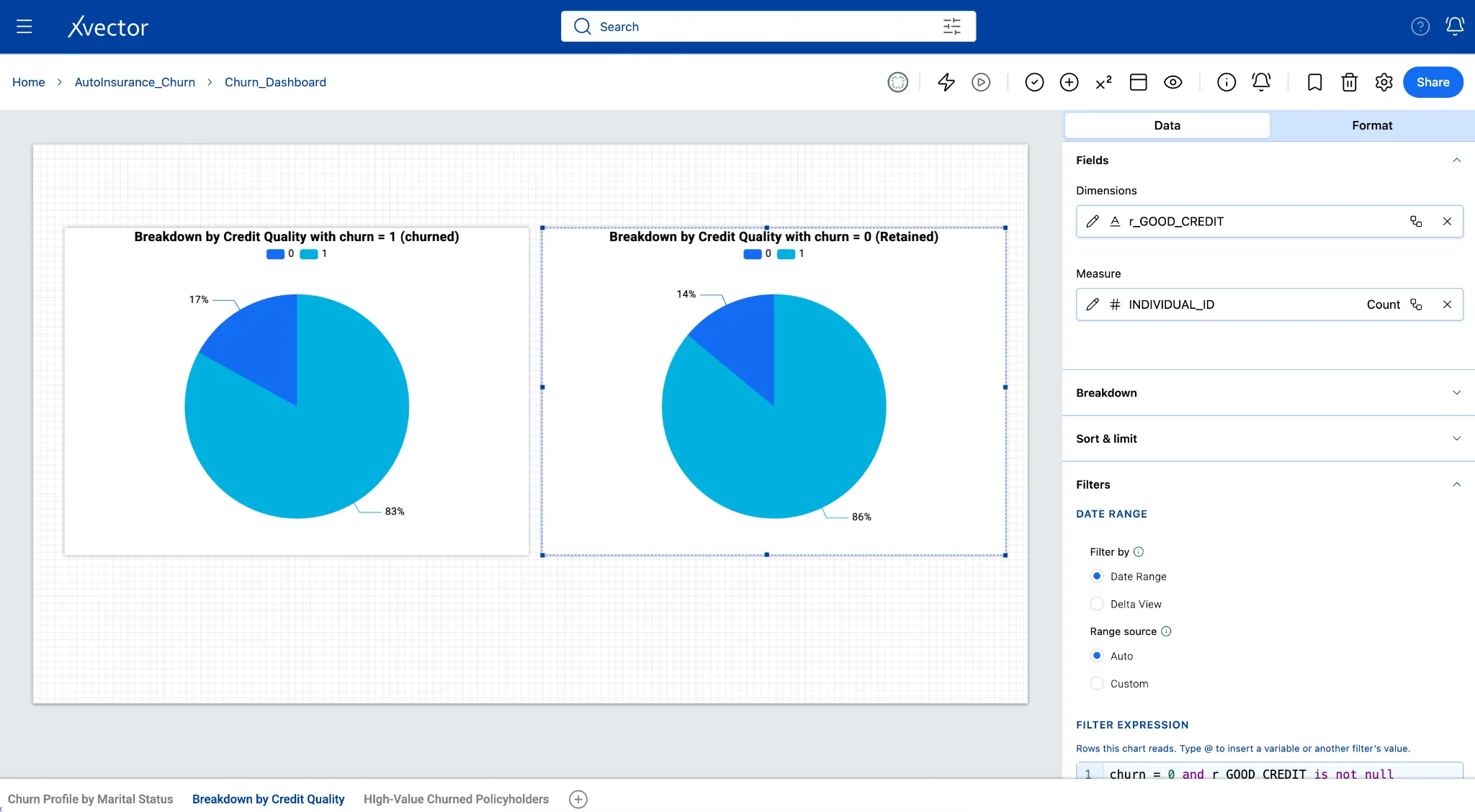
The side-by-side pie charts compare the proportion of policyholders with good credit (r_GOOD_CREDIT = 1, shown in light blue) versus poor or fair credit (r_GOOD_CREDIT = 0, shown in dark blue) across two distinct groups: churned customers on the left (churn = 1) and retained customers on the right (churn = 0). By measuring the count of unique individuals (INDIVIDUAL_ID count) in each segment, the charts show whether credit quality drives policy attrition as an underlying financial risk factor.

1. Click the + icon next to the sheet tab. Name the new sheet Breakdown by Credit Quality.

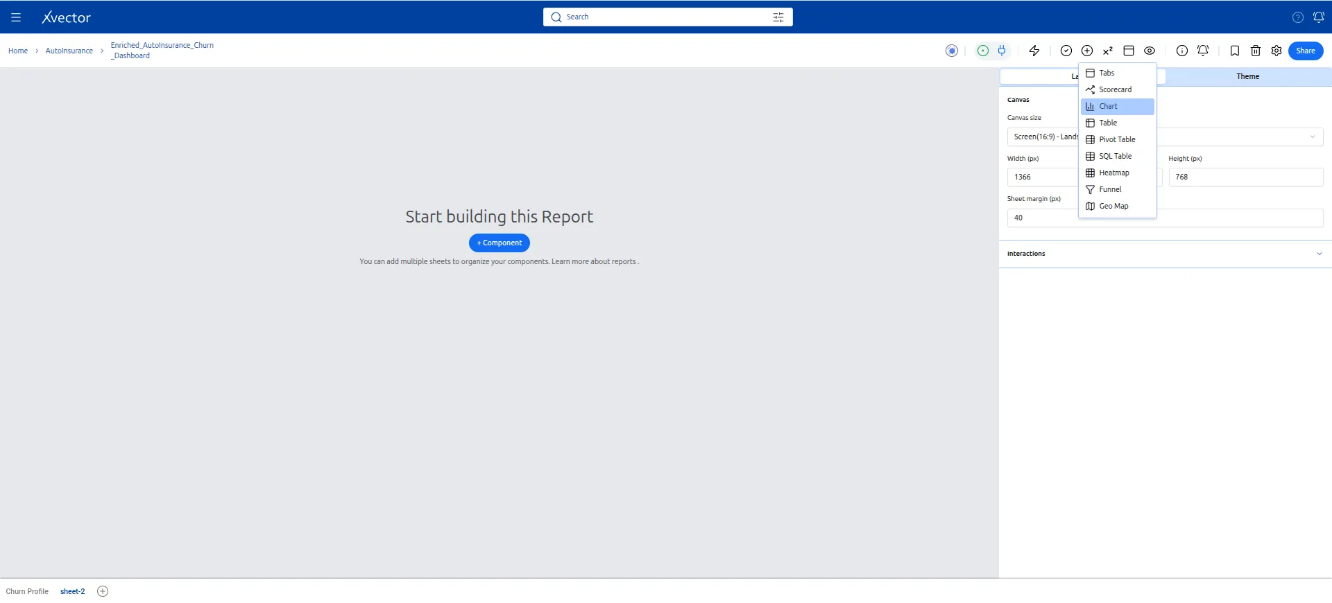
2. Click Add Component (+) and select Pie Chart.

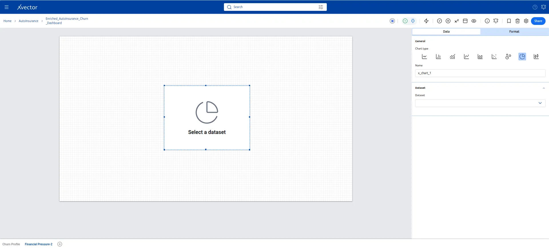
3. Configure the first pie chart (Churned customers):

Setting	Value
Dataset	Customer_Churn
Dimension	r_GOOD_CREDIT
Measure	INDIVIDUAL_ID (count)
Filter on component	churn = 1
Title	Breakdown by Credit Quality with Churn = 1 (Churned)

Filter: Churn=1 and good_credit is not null

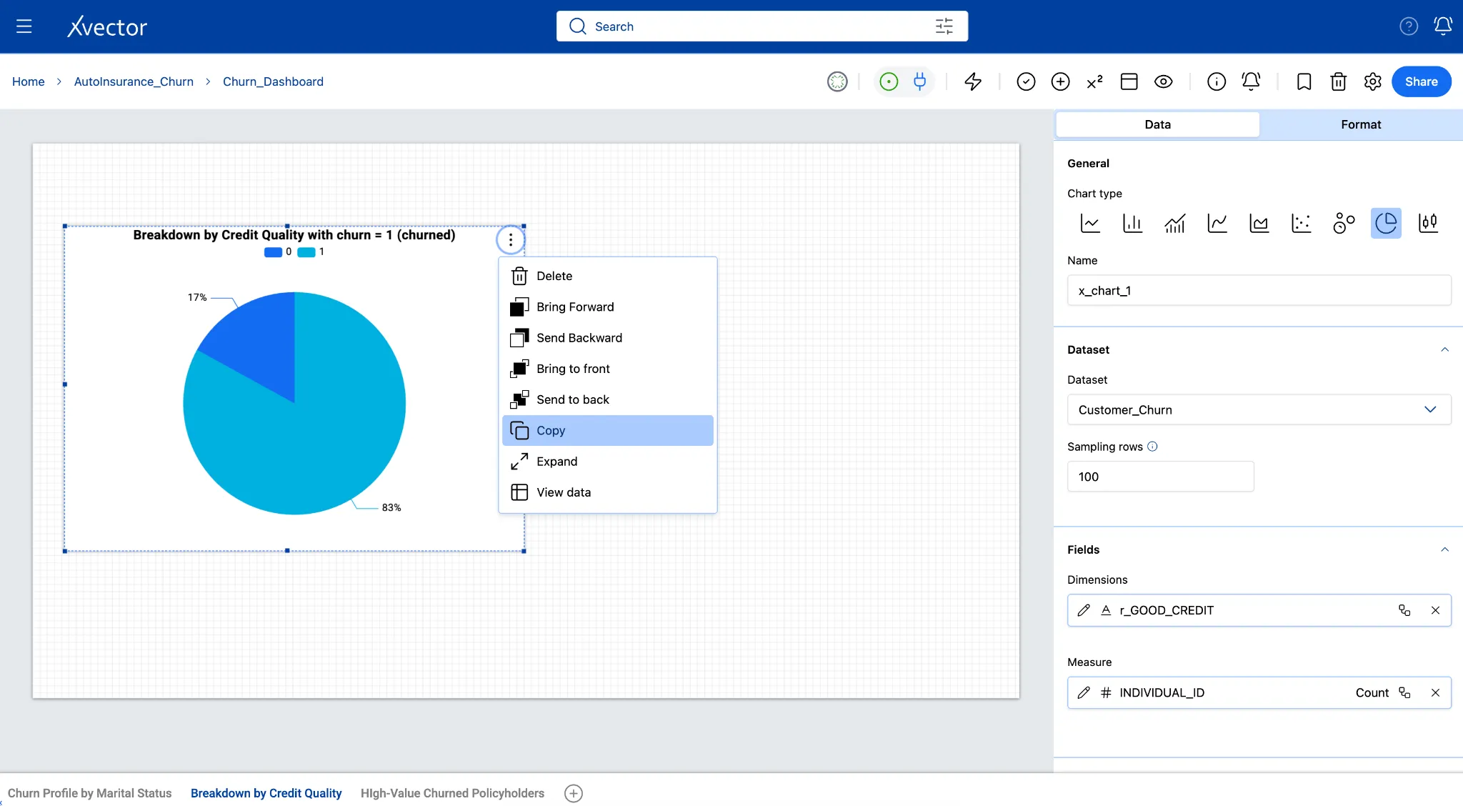
4. Copy the component (three-dot menu → Copy) and paste (Ctrl+V or Cmd+V) next to the first. Update the title to “Breakdown by Credit Quality with Churn = 0 (Retained)”.

Filter: Churn=0 and good_credit is not null

5. Place both charts side by side for direct comparison.

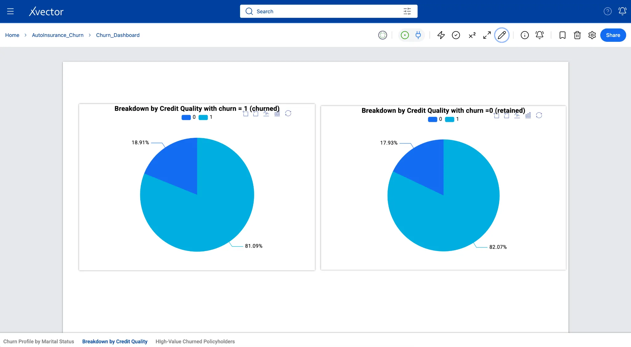
In this view, churned customers show an 83% to 17% split, closely mirroring the 86% to 14% split in retained customers, indicating that credit tier alone does not strongly skew cancellation rates in this dataset.

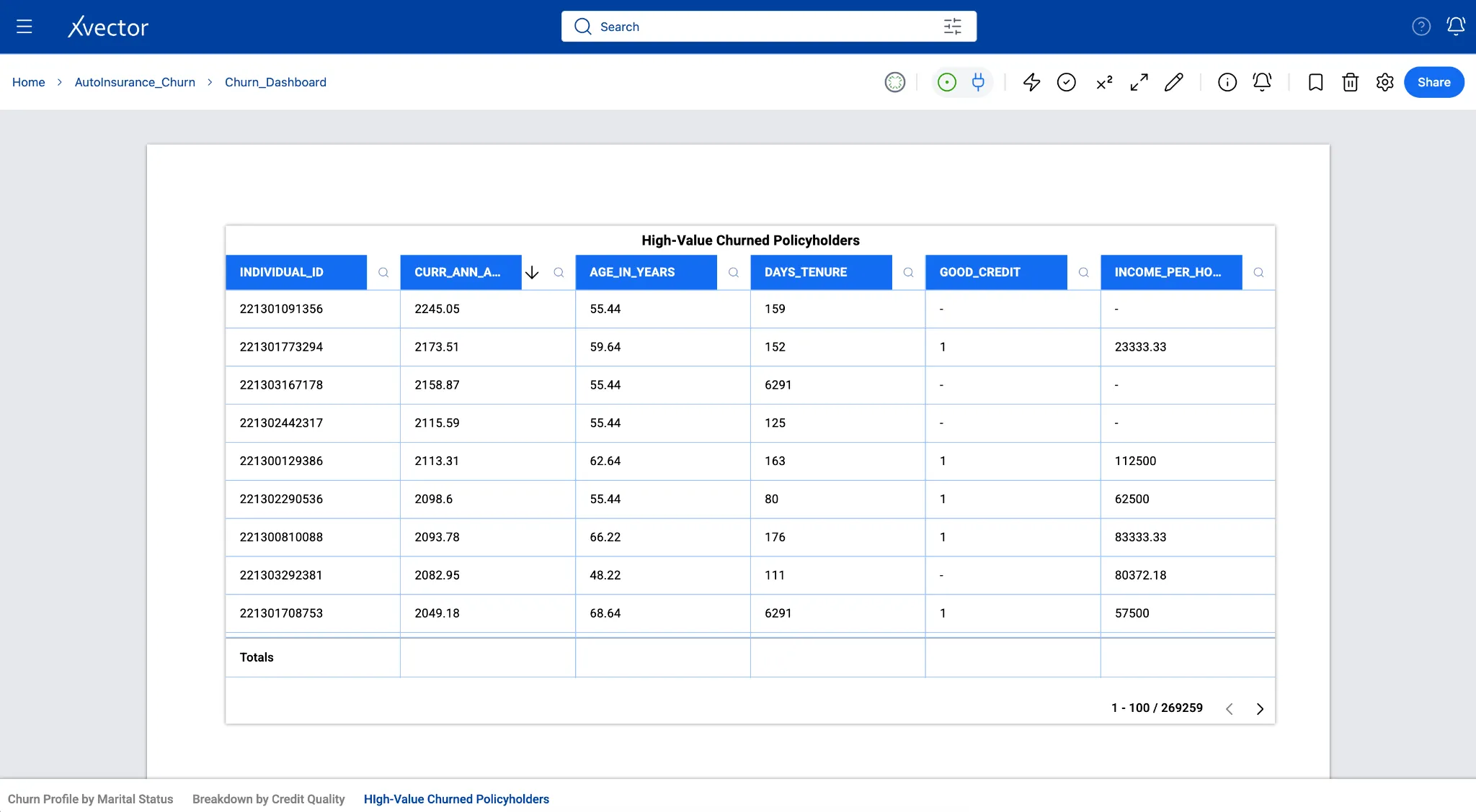
Sheet 3 - High-Value Churned Customers (Table)

Business question: Which high-value churned customers should we act on first?

Not all churned customers represent the same revenue loss. Prioritizing retention efforts on high-premium, long-tenure, good-credit customers - the ones most worth winning back - is a better use of a retention team’s time than treating all churn equally. This table surfaces those customers in priority order, with the columns an account manager needs to decide.

A table sorted by annual premium (descending) surfaces the highest-value churned accounts, those with the greatest revenue impact. This helps operations or underwriting teams take action.

1. Click the + icon. Name the new sheet Action List.

2. Click Add Component (+) and select Table.

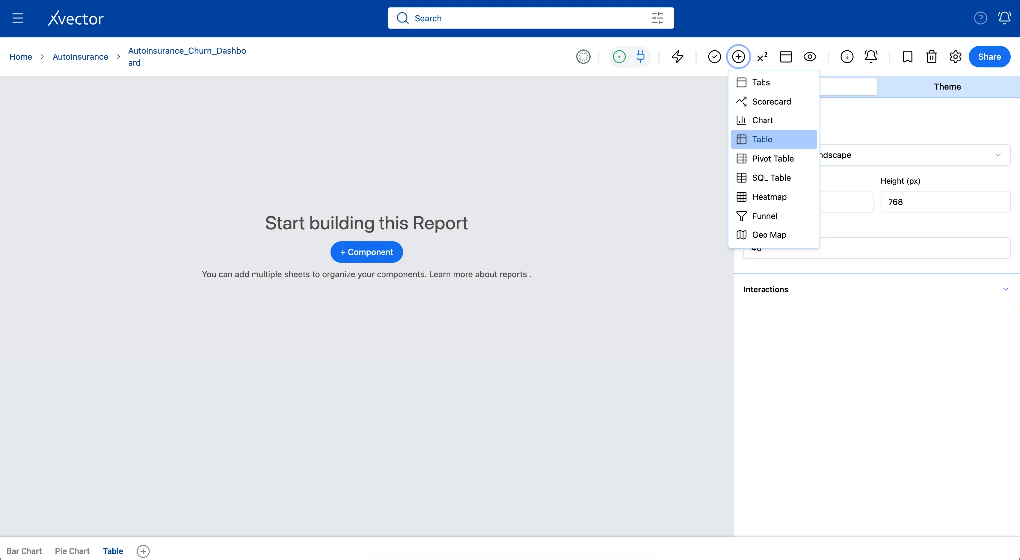
3. Update the Data tab with the following:

Setting	Value
Dataset	Customer_Churn
Filter on component	churn = 1 (churned policyholders only)
Sort	curr_ann_amt descending

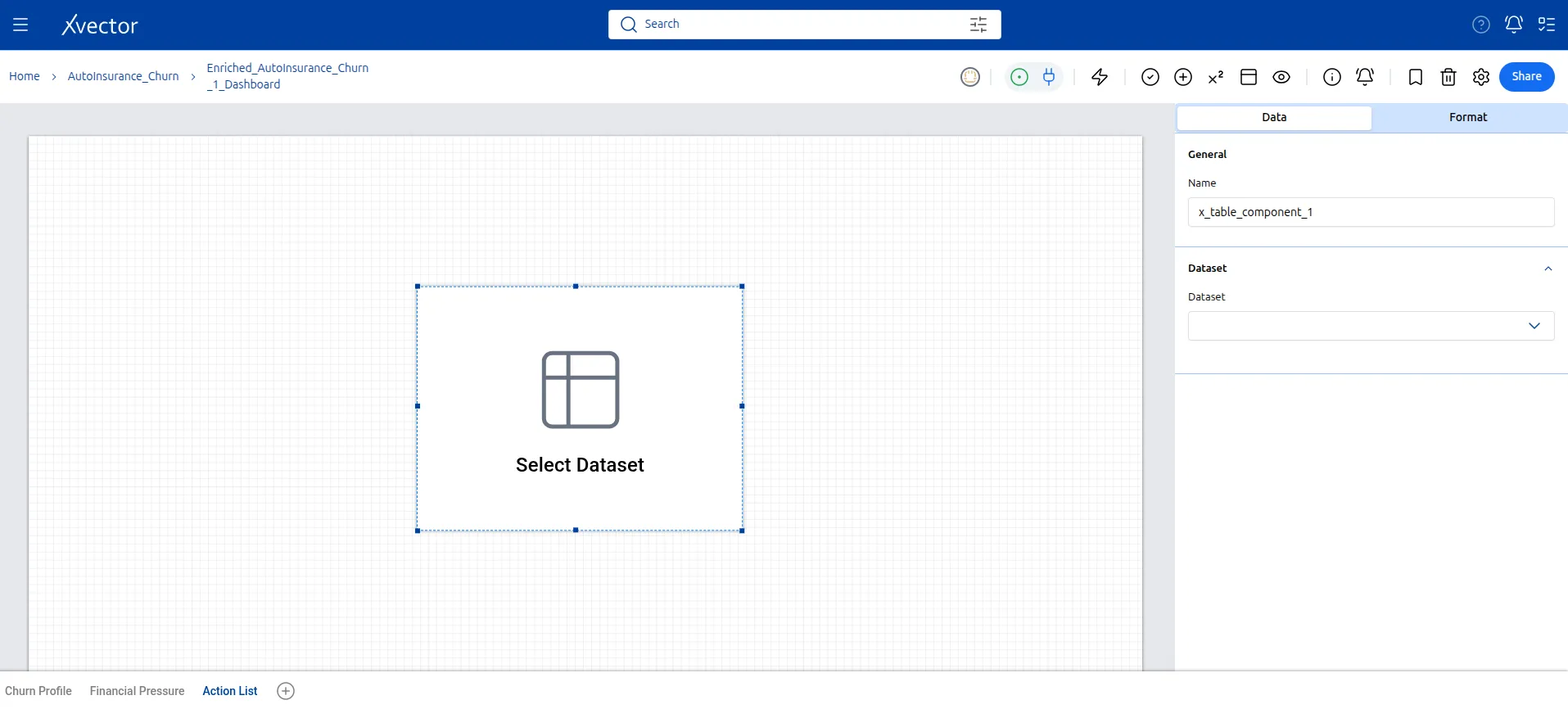
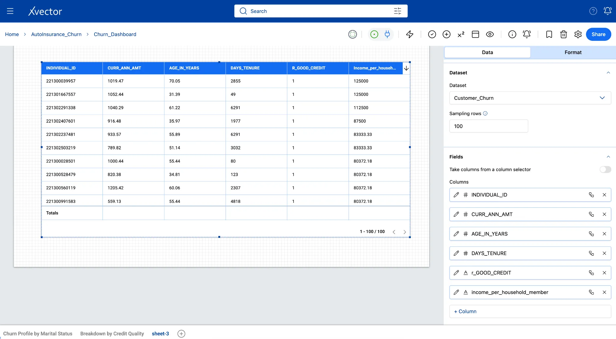
4. Select these columns to display:

Individual_id, curr_ann_amt, age_in_years, days_tenure, good_credit, income_per_household_member

5. In the Format tab, title it High-Value Churned Policyholders.

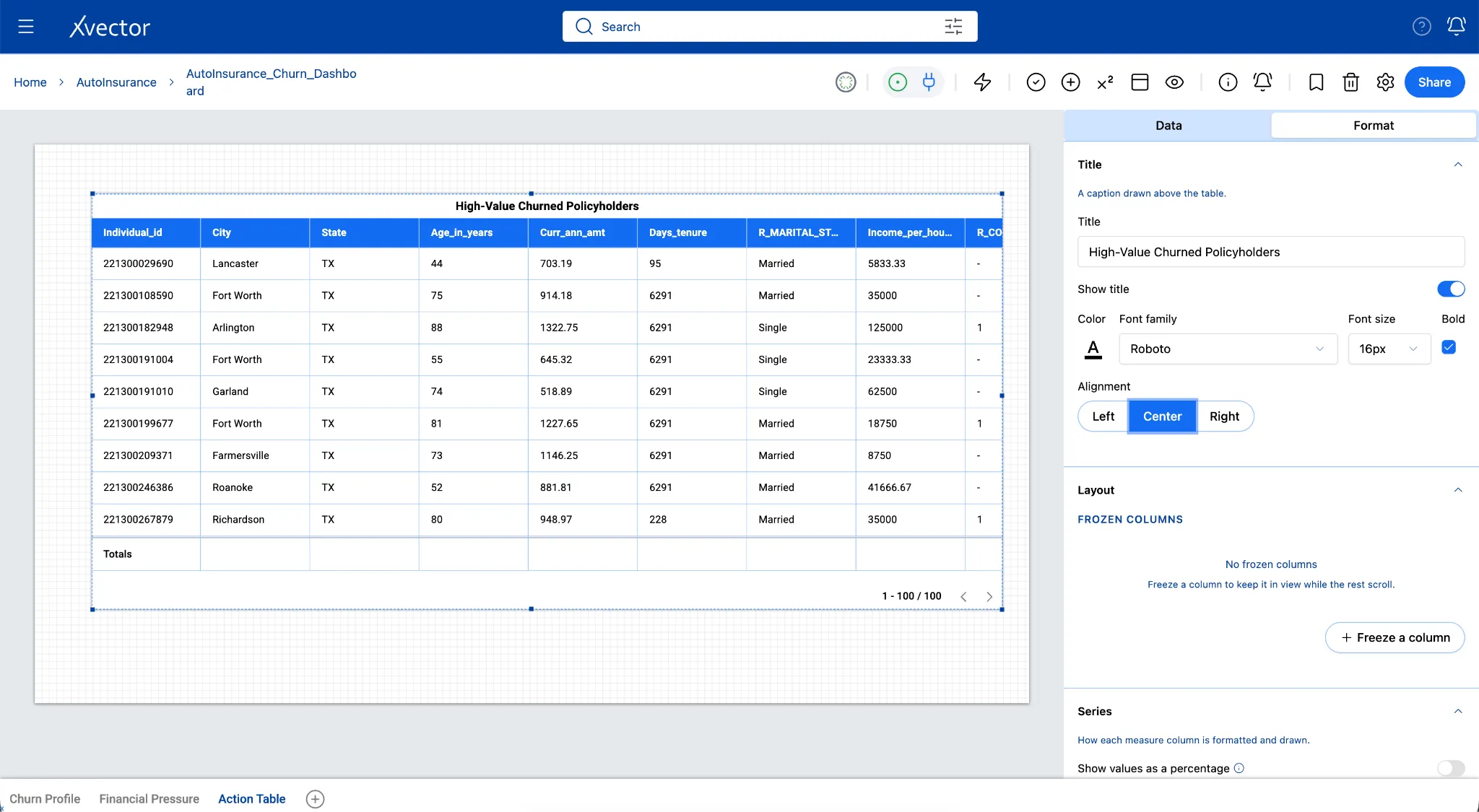
How to read this table:

Pattern in the row	What it may mean
good_credit = 1 and churned	Low-risk customer who left; high priority for a win-back call
High curr_ann_amt + low income_per_household_member	Premium may be genuinely unaffordable relative to household size
days_tenure over 3,000 (~8 years) and churned	Long-loyal customer who left after something changed; worth investigating

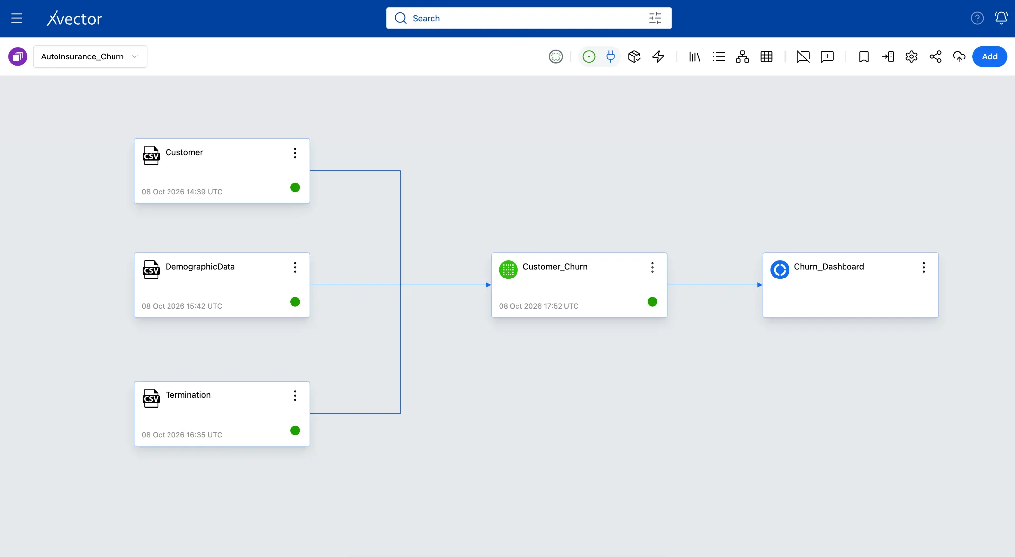
Here’s the final workspace with the following resources:

• 3 Datasources

• 1 Dataset

• 1 Report with 3 sheets