Analyst Handbook
The Analyst Handbook serves as a guide for analysts to perform exploratory data analysis and extract actionable insights using simple models within the xVector Platform. It also provides insights into orchestration and observability within data workflows. The handbook uses four business cases, tied to key modeling approaches (Regression, Classification, Clustering, and Time Series), to contextualize these concepts, with a focus on Marketing Analytics applications.
-
The first business case focuses on marketing campaign and sales data. It uses linear regression to optimize marketing spend across different advertising channels and maximize sales revenue. The company’s historical data on marketing campaigns and sales figures is explored to identify which channels provide the best ROI and determine the expected sales impact.
-
The second business case involves optimizing marketing strategies for a bank. It uses a random forest classification model to analyze bank marketing data to identify factors that drive campaign success and target customer segments that are most likely to respond positively.
-
The third business case aims to identify and understand customer segments based on purchasing behaviors. It uses KMeans clustering to analyze online retail transaction data to improve customer retention and maximize revenue by understanding customer segments and their purchasing behaviors.
-
The fourth business case involves analyzing and forecasting sales trends using store sales data. It uses an ARIMA time series model to identify peak sales periods, understand growth trends, and uncover seasonal patterns to optimize inventory, plan promotions, and enhance revenue predictability.
These business cases, taken from kaggle, will help you get familiar with the xVector Platform.
The handbook provides information on evaluating metrics and model comparison, and discusses topics such as data exploration and data snooping.
Advanced modeling techniques, evaluations, and ML operations are discussed in Data Scientist Handbook.
Data operations such as data quality, pipelines, and advanced enrichment functions are covered in the Data Engineering Handbook.
xVector Platform Overview
Section titled “xVector Platform Overview”xVector is a unified platform for building data applications and agents powered by a MetaGraph. Users can bring in data from various sources, enrich the data, explore, apply advanced modeling techniques, derive insights, and act on them, all in a single pane, collaboratively.
Business Case 1 (Regression): Marketing Campaign and Sales Data
Section titled “Business Case 1 (Regression): Marketing Campaign and Sales Data”Consider a business that would like to optimize marketing spend across different advertising channels to maximize sales revenue. This involves determining the effectiveness of TV, social media, radio, and influencer promotions in driving sales and understanding how to allocate budgets for the best return on investment (ROI).
The company has historical data available on the marketing campaigns, including budgets spent on TV, social media, radio, and influencer collaborations, alongside the corresponding sales figures. However, the question remains: how can the company predict sales more accurately, identify which channels provide the best ROI, and determine the expected sales impact per $1,000 spent?
This journey begins by exploring the data, which includes sales figures and promotional budgets across different channels. Raw data is rarely in a usable form right from the start. We address potential biases, handle missing values, and identify outliers that could distort the results. With a clean and well-prepared dataset, the next step is to dive deeper into the data to extract meaningful insights.
To make informed decisions on marketing spend, businesses need to understand how each advertising channel influences sales. The relationship between marketing spend and sales is complex, with many factors at play. By fitting a linear regression model to the data, we can estimate how changes in the marketing budget for each channel influence sales. This helps identify which channels yield the highest sales per dollar spent and provides a framework for making more informed budget allocation decisions. For instance, the model might show that spending on TV ads yields the highest return on investment, while spending on social media or radio could be less effective, guiding future budget allocations.
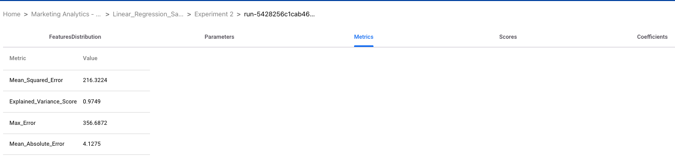
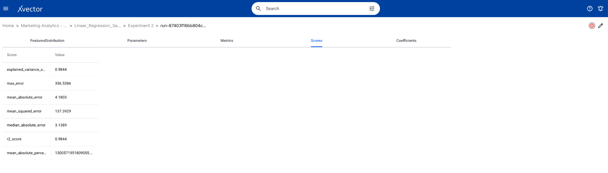
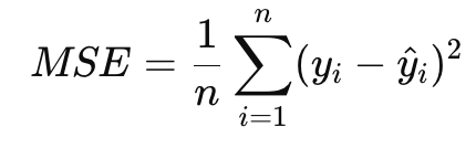
Having identified effective channels, it is important to ensure the accuracy and reliability of the predictions. R² and Mean Squared Error are measures of the model’s performance. R² score, in particular, indicates how well the model explains the variance in sales based on marketing spend, with a higher score suggesting that the model can predict sales more accurately. On the other hand, the Mean Squared Error (MSE) measures the average squared difference between predicted and actual sales, helping to assess the quality of the predictions — lower MSE values indicate a better fit of the model to the data.
By evaluating these metrics, businesses gain confidence in the model’s ability to make reliable predictions. With these insights, companies can fine-tune their marketing strategies, reallocate budgets to the highest-performing channels, and identify areas where additional investment may not yield optimal results.
Now, let us look at how all this can be achieved in the xVector Platform.
Dataset Overview
Section titled “Dataset Overview”You can download the Marketing Campaign and Sales Data from kaggle. This data contains:
- TV promotion budget (in million)
- Social Media promotion budget (in million)
- Radio promotion budget (in million)
- Influencer: Whether the promotion collaborates with Mega, Macro, Nano, Micro influencer
- Sales (in million)
Analysis Questions:
- Which advertising channel provides the best ROI?
- How accurately can we predict sales from advertising spend?
- What’s the expected sales impact per $1000 spent on each channel?
Importing Data
Section titled “Importing Data”xVector has a catalog of connectors. If required, you can build connectors to custom sources and formats.
Below are the steps to implement this in the xVector Platform:
Understanding the Dataset
Section titled “Understanding the Dataset”Once the data is imported, create a dataset for enrichment purposes. xVector provides the capability to keep these datasets synchronized with the original data sources, ensuring consistency.
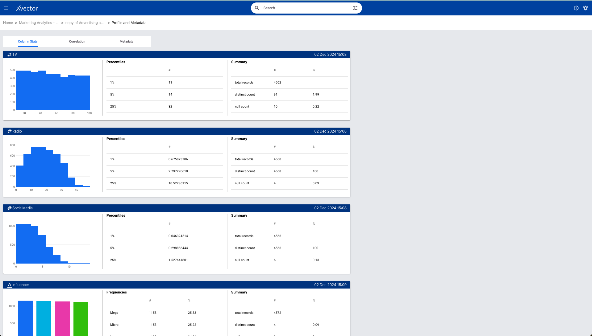
Data exploration (suggested checklist) entails understanding the process that generates the data and the characteristics of the data. In this case, the process refers to the marketing department’s spending on various channels, as captured in the systems. As for some of the data characteristics, the dataset has very few missing values. The social media column has only six missing values out of around 4570 records. These records can either be removed or populated with average values or values provided by the business user from another system, etc. Influencer is a categorical value, and there are 4 unique values for this column.
xVector provides out-of-the-box tools to profile the data. To explore the data further, you can create reports manually or by using the GenAI-powered options. Generate Exploratory Report and Generate Report are GenAI reports built on the platform.
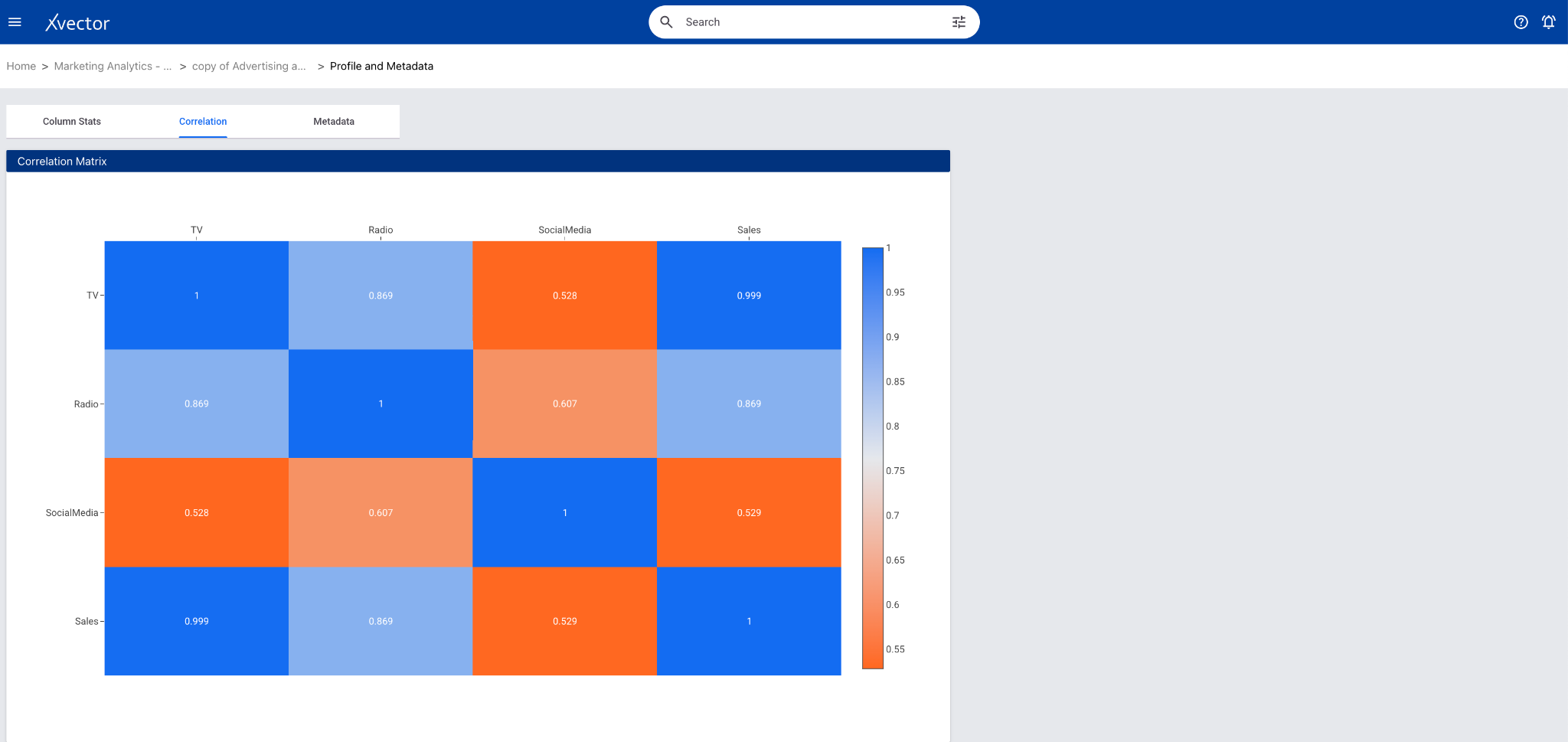
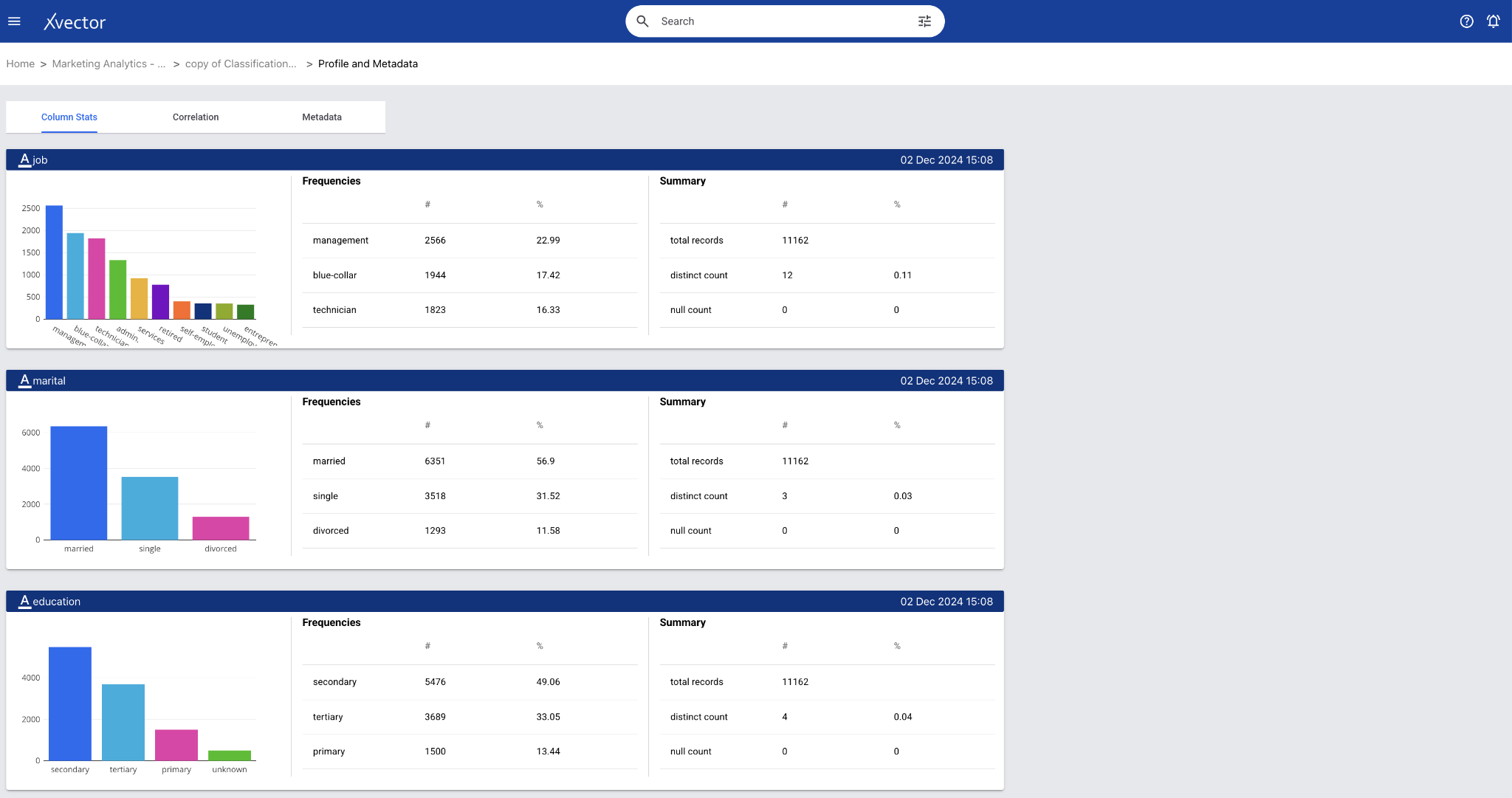
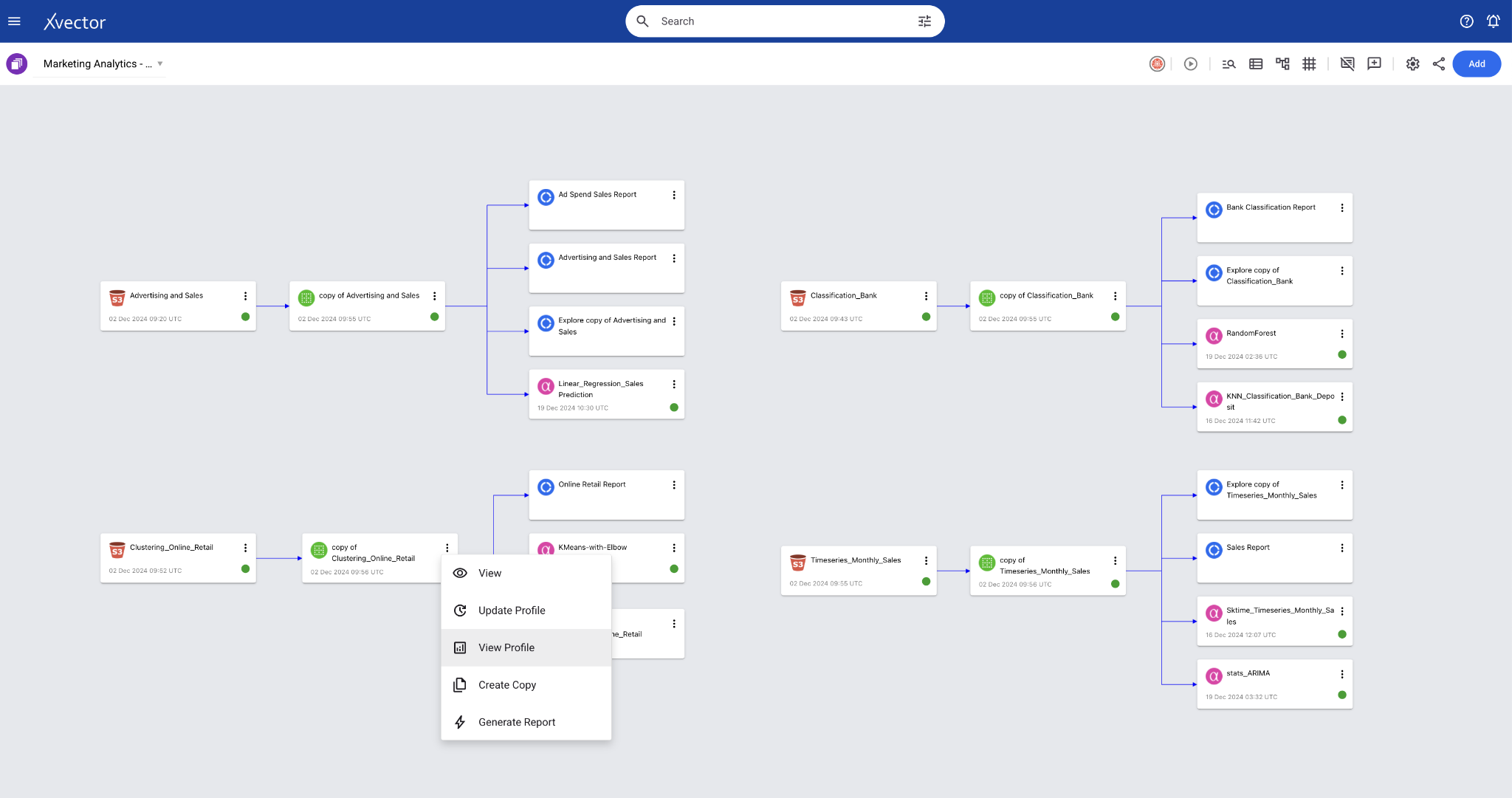
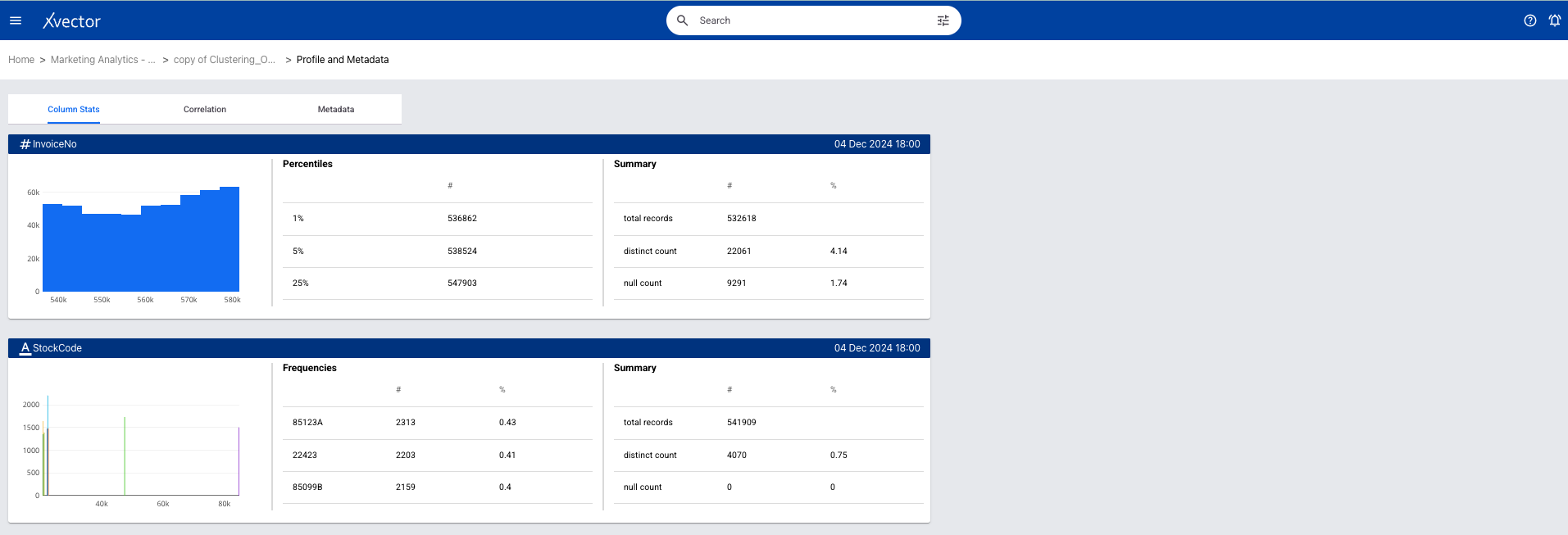
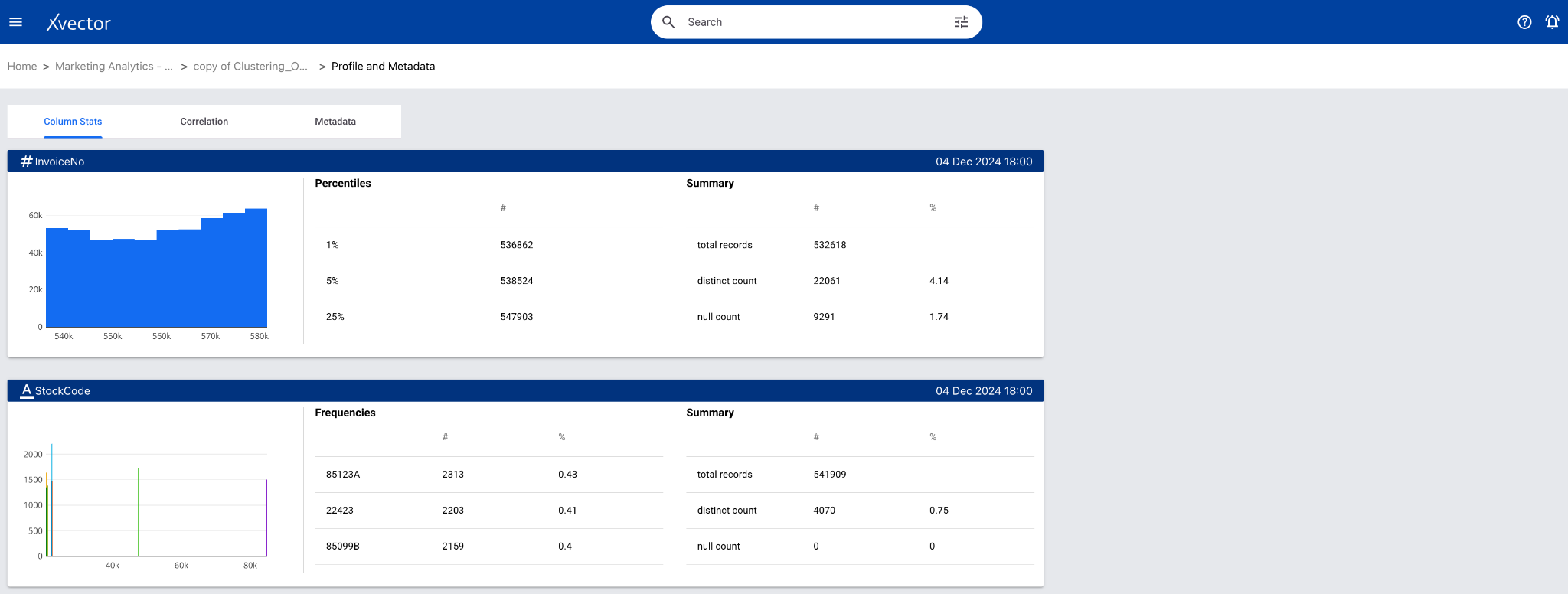
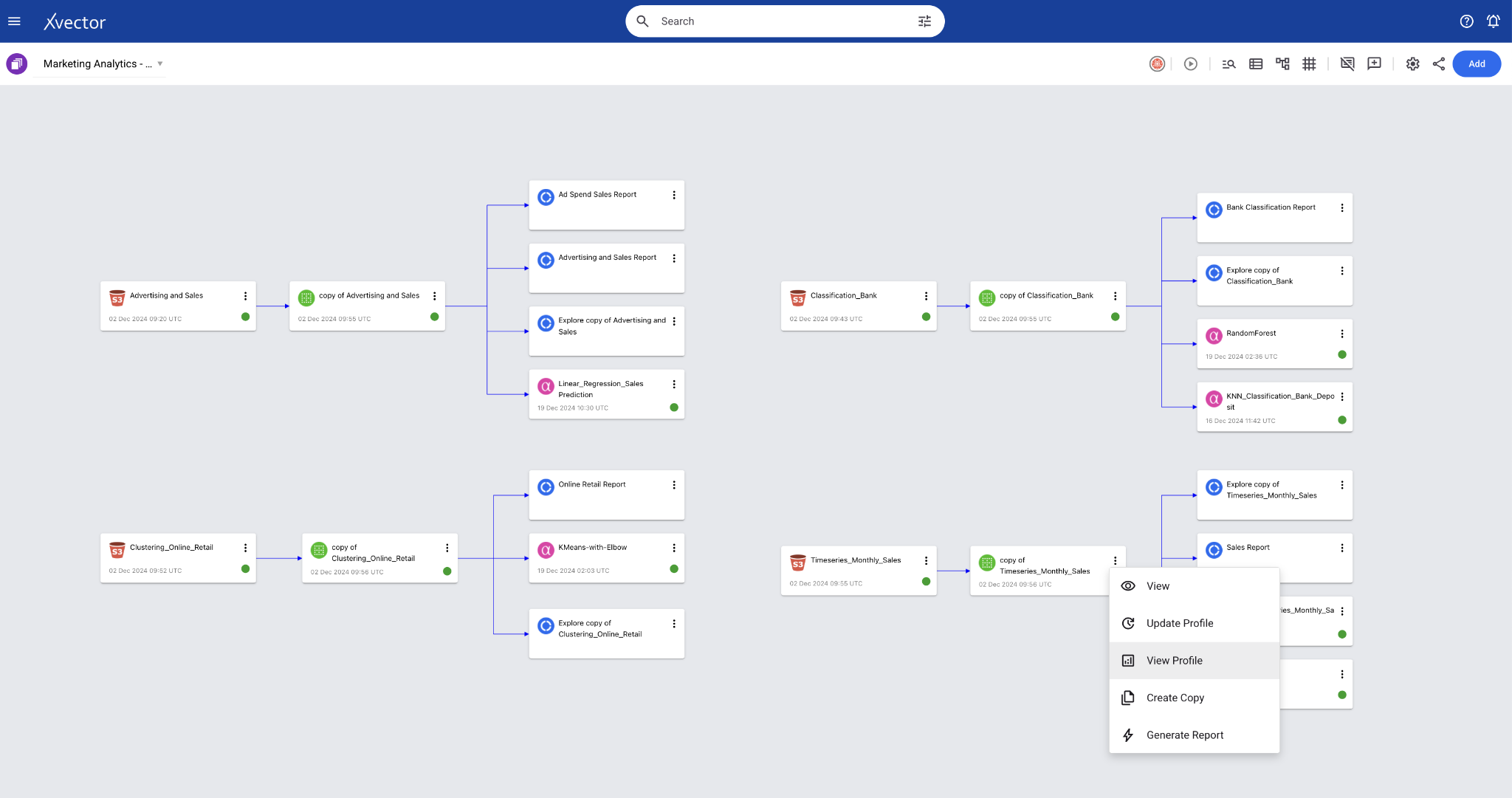
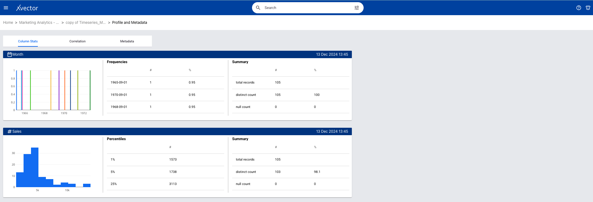
To view the data profile page, click on the kebab menu (vertical ellipses) → “View Profile” on the created dataset. Profile view helps identify outliers and correlations.
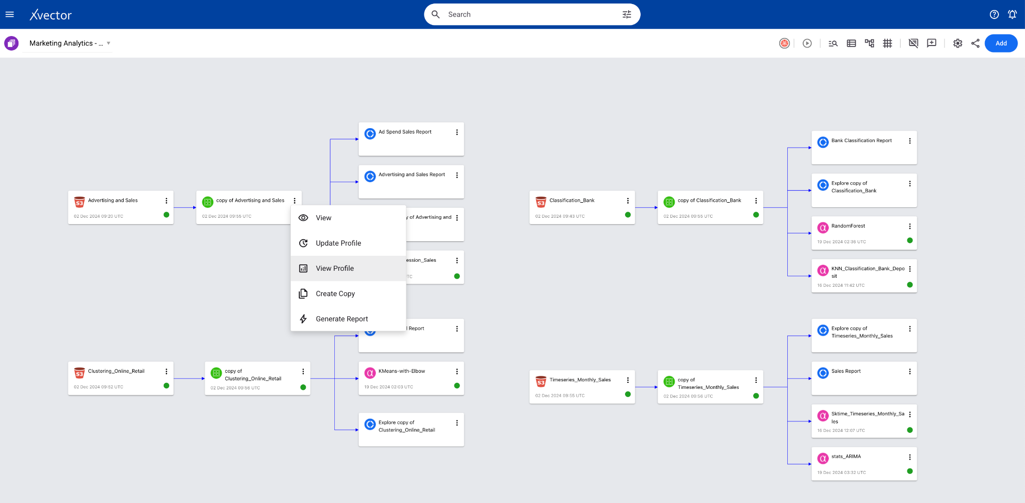
Below is the profile page view of the dataset:
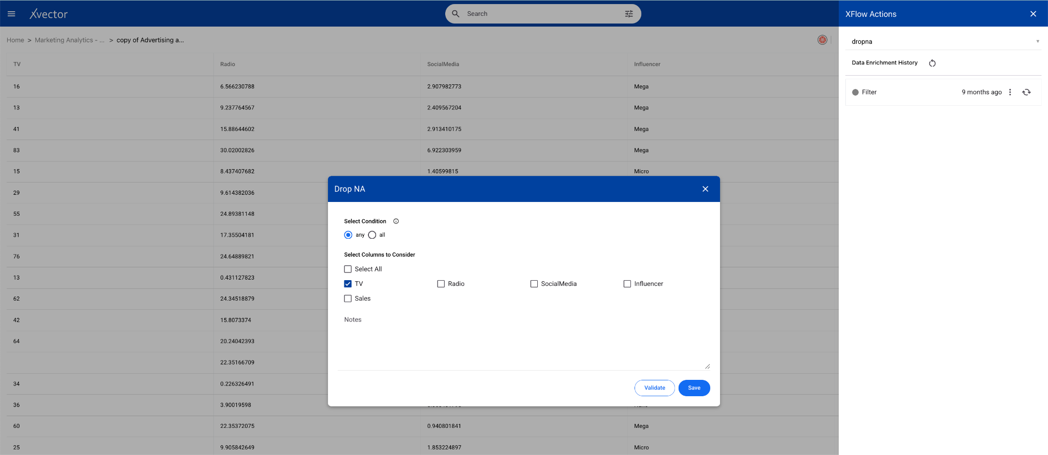
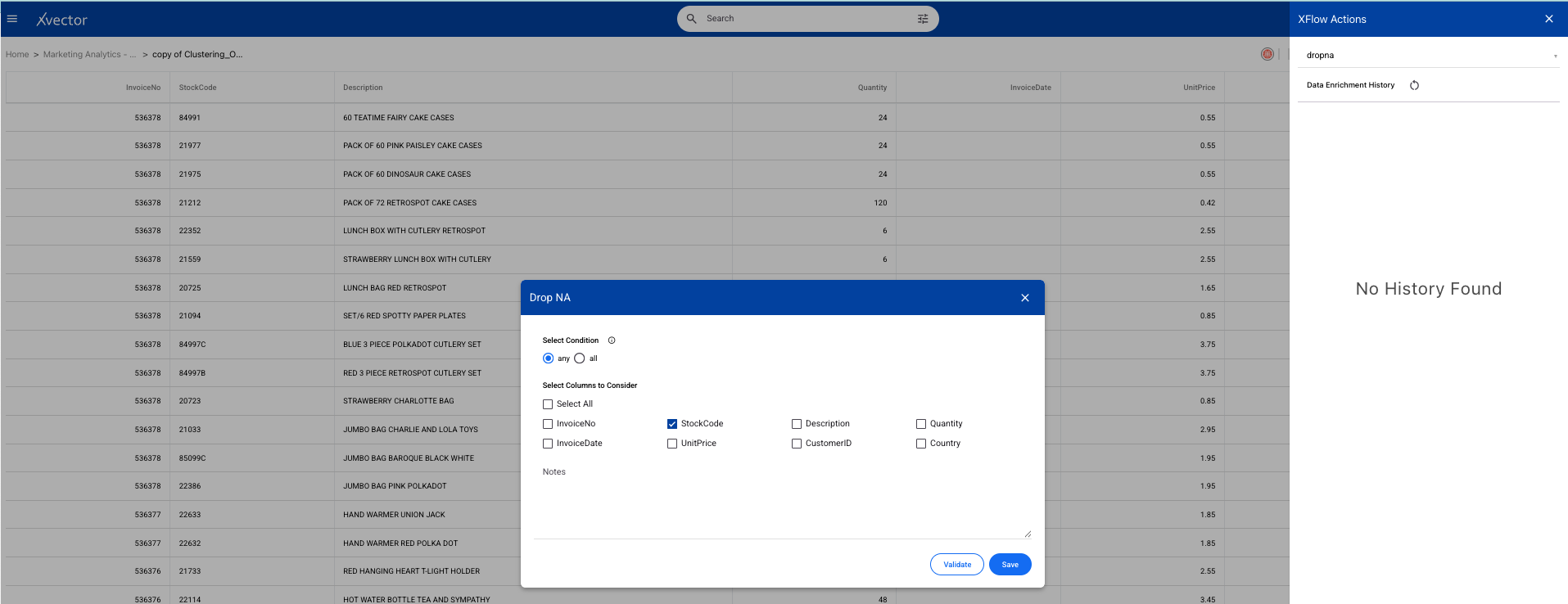
Once you perform basic exploration of the data, you can then enrich the data. For example, “dropna” is one such function used to drop records with null values.
Maximizing Sales Revenue
Section titled “Maximizing Sales Revenue”In the current case, the business would like to optimize marketing spend across different advertising channels to maximize sales revenue. Using the regression model, we can predict sales based on various input factors (such as TV, social media, radio, and influencer spend).
Implementing the Solution
Section titled “Implementing the Solution”Having created the dataset and explored the data, we are now ready to build a linear regression model to analyze and make predictions.
In the world of xVectorlabs, each model is a hub of exploration, where experiments are authored to test various facets of the algorithm. A user can create multiple experiments under a model. An experiment includes one or more runs. Under each experiment, various parameters with available drivers can be tried on different features.
Experiments can have multiple runs with different input parameters and performance metrics as output. Based on the metric, one of these runs can be chosen for the final model.
The platform provides a comprehensive set of model drivers curated based on industry best practices. Advanced users can author their custom drivers, if required.
For the current dataset, we will use an existing model driver, Sklearn-LinearRegression. Follow the steps to build a linear regression model and use the model Sklearn-LinearRegression. Use appropriate parameters and evaluation metrics to optimize the solution.
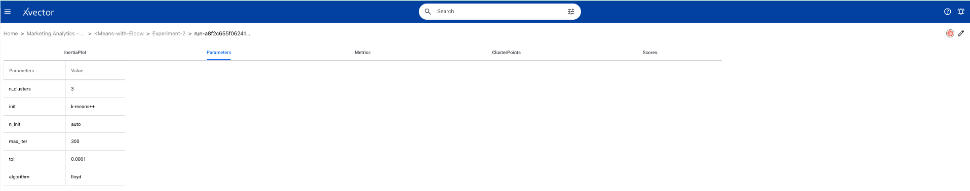
Here is a linear regression model implemented in xVector.
The below run shows the parameters used along with the metrics and scores for analysis.
Analysis
Section titled “Analysis”Which Advertising Channel provides the best ROI?
-
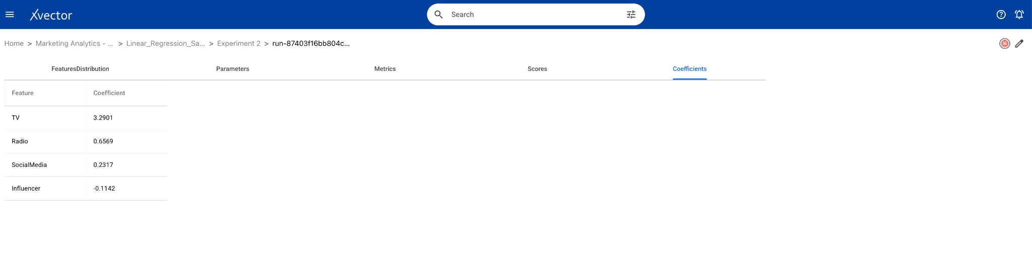
The channel with the highest positive coefficient in the regression model has the greatest impact on sales per dollar spent. In linear regression, coefficients are numerical values that represent the relationship between predictor variables and the response variable. They indicate the strength and direction of the relationship and are multiplied by the predictor values in the regression equation. A positive coefficient means that as the predictor increases, the response variable also increases, while a negative coefficient indicates an inverse relationship.
-
In the above example, TV provides the best ROI as TV has the max. coefficient of 3.29.
This can also be inferred from the correlation matrix in the profile page of the dataset. In this case TV has the maximum correlation which is 0.99.
How accurately can we predict sales from Advertising Spend?
- The R² score measures the proportion of variance in sales explained by advertising spend. Closer to 1 implies high accuracy.
- In the above example, it is quite accurate as R² score is 0.98
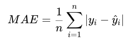
- The Mean Absolute Error (MAE) quantifies the average error between actual and predicted sales. A lower MAE indicates that the model’s predictions are closer to the actual values.
- Mean Absolute Error is 4.18, which is low implying the predictions are closer to the actual values.
What’s the Expected Sales Impact per $1000 spent on each Channel?
- Use the Impact per $1000 column from the coefficients DataFrame.
- The coefficient of TV is 3.2938. This predicts that spending $1000 more on TV ads is expected to increase sales by $3293.8.
Negative Coefficients
- A negative coefficient suggests an inverse relationship between the corresponding feature and the outcome variable. Specifically:
- Influencer (-0.1142): Spending $1000 on Micro-Influencers reduces the outcome by roughly $114.20.
Possible Explanations for Negative Impacts:
- Diminishing Returns: These marketing channels might already be saturated, leading to diminishing or negative returns on additional investment.
- Ineffective Strategy: The investment in these areas may not be optimized, or the target audience might not respond well to these channels.
- Indirect Effects: The spending might be cannibalizing other channels or producing unintended negative outcomes (e.g., customer annoyance, ad fatigue).
Business Case 2 (Classification): Bank Marketing Dataset
Section titled “Business Case 2 (Classification): Bank Marketing Dataset”The objective of the Bank is to maximize Term deposits from customers by optimizing marketing strategies. This can be done by identifying the factors that drive campaign success, understanding the overall campaign performance, and targeting customer segments most likely to respond positively.
First, we explore the dataset, which contains customer demographics, past campaign data, and behavioral features such as job, education, and balance. The current dataset has 10 categorical columns: marital status, education, and job.
To predict whether a customer will subscribe to a term deposit, we use the Random Forest classification model. This model is chosen for its ability to handle complex, non-linear relationships between features and the ability to provide feature importance rankings to identify the most influential predictors.
By continuously validating and refining the model, the bank ensures its marketing campaigns remain data-driven, efficient, and impactful, leading to improved conversion rates and better resource allocation.
Dataset Overview
Section titled “Dataset Overview”You can download the Bank Marketing Dataset from kaggle.
The Bank tracks customer term deposits along with their attributes in their systems. The dataset has 10 categorical features including Age, Marital Status, Job, Loan, Education, term deposit etc. There are 12 distinct job categories and 3 distinct marital status categories.
Analysis Questions:
- What factors best predict campaign success?
- What’s the overall campaign success rate? **
** To be done in the Data Scientist Handbook
Importing Data
Section titled “Importing Data”Understanding the Data
Section titled “Understanding the Data”Once the data is imported, create a dataset for enrichment purposes. xVector provides the capability to keep these datasets synchronized with the original data sources, ensuring consistency.
Data exploration (suggested checklist) entails understanding the process that generates the data and the characteristics of the data. The Bank Marketing dataset includes 17 attributes, with features such as customer demographics (e.g., age, job, marital status, education), financial details (e.g., balance, loan, housing), and engagement data (e.g., previous campaign outcomes, duration of calls, and contact methods). The target variable, deposit, indicates whether the customer subscribed (yes or no). The age range for this dataset is between 18 and 95 with about 57% of them being married.
The dataset also has negative amounts as balance for a few records. Depending on how the bank is tracking balances, it is possible that these customers have withdrawn more than what’s available in their account. So, we shouldn’t drop these records without understanding how the Bank tracks balances.
xVector provides out-of-the-box tools to profile the data. Generate Report and Generate Exploratory Report are GenAI reports built on the platform.

Once you perform basic exploration of the data, you can then enrich the data. For example, “dropna” is one such function used to drop records with null values.
Maximizing Term Deposit Subscriptions
Section titled “Maximizing Term Deposit Subscriptions”We can use the classification model due to its ability to handle complex, non-linear relationships between features and the ability to provide feature importance rankings to identify the most influential predictors.
Implementing the Solution
Section titled “Implementing the Solution”For the current dataset, we will use an existing model driver, RandomForest. Follow the steps to build a classification model and use the model driver RandomForest. Use appropriate parameters and evaluation metrics to optimize the solution.
Here is a classification model implemented in xVector.

Analysis
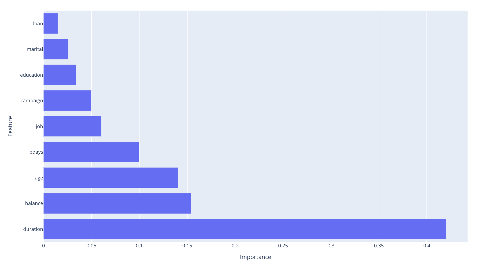
Section titled “Analysis”What factors best predict campaign success?
Feature importance from the Random Forest model reveals the most influential factors. In this case, the top 3 features are duration, balance, and age.
**What’s the overall campaign success rate? ****
The proportion of deposit == ‘yes’ gives the success rate. Here, the overall Campaign Success Rate is 47.38%
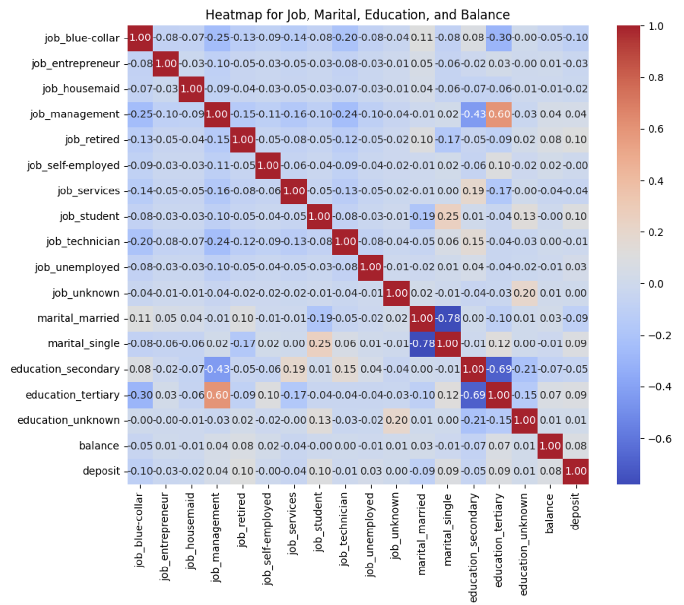
**Which customer segments are most likely to respond positively? ****
Based on the heatmap below, those with management jobs and tertiary education are most likely to respond positively.
Business Case 3 (Clustering): Online Retail Transaction Data
Section titled “Business Case 3 (Clustering): Online Retail Transaction Data”An online retail store would like to identify and understand customer segments based on purchasing behaviors to improve customer retention and maximize revenue. By distinguishing the most valuable customers, the company can create targeted marketing strategies, enhance loyalty programs, and optimize resource allocation to increase long-term profitability.
The Online Retail Transaction dataset includes transactional details such as invoice numbers, stock codes, product descriptions, quantities, invoice dates, and customer IDs, along with the country of purchase. The primary goal is to use this information to segment customers based on their purchase behavior and determine which segments represent the most valuable customers.
The analysis begins with data exploration and preparation, a critical step for ensuring accuracy and reliability. Once the data is cleaned and enriched, the focus shifts to determining the optimal number of groups for segmentation using the elbow method. The final step is to analyze the features that are most important for grouping or segmenting the dataset.
Dataset Overview
Section titled “Dataset Overview”You can download the Online Retail Transaction Data Source from Kaggle.
This dataset includes transactional details such as invoice numbers, stock codes, product descriptions, quantities, invoice dates, customer IDs, unit price, and the country of purchase. Out of the 38 countries, UK far exceeds the others in sales of these products.
Analysis Questions:
- Are there outliers in the data points?
- What should be the number of groups to segment the data points?
- What are the important features to consider while grouping or segmenting dataset?
Importing Data
Section titled “Importing Data”Understanding the Data
Section titled “Understanding the Data”Once the data is imported, create a dataset for enrichment purposes. Data exploration (suggested checklist) entails understanding the process that generates the data and the characteristics of the data. The Online Retail Transaction dataset contains records of customer purchases. There are several records with negative quantity which are not valid values. The invoices range between December 2010 and December 2011. Around 500K records belong to United Kingdom.
xVector provides out-of-the-box tools to profile the data. Generate Exploratory Report and Generate Report are GenAI reports built on the platform.
Once you perform basic exploration of the data, you can then enrich the data. For example, “dropna” is one such function used to drop records with null values.
Here is a link to the Profile page on an xVector DataApp:
Customer Segmentation to Maximize Revenue
Section titled “Customer Segmentation to Maximize Revenue”The K-Means clustering model is ideal for this dataset as it effectively segments customers into meaningful groups based on their purchasing behavior, uncovering patterns in the data.
For the current dataset, we will use an existing model driver, KMeans-with-Elbow. Follow the steps to build a KMeans Clustering model and use the model driver KMeans-with-Elbow. Use appropriate parameters and evaluation metrics to optimize the solution.
Here is a KMeans Clustering model implemented in xVector.
Analysis
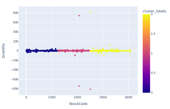
Section titled “Analysis”Are there any outliers in the data points?
Using KMeans clustering, we can detect unusual patterns in transaction amounts or quantities. In the current dataset, we only see a very sparse set of datapoints that are outliers:
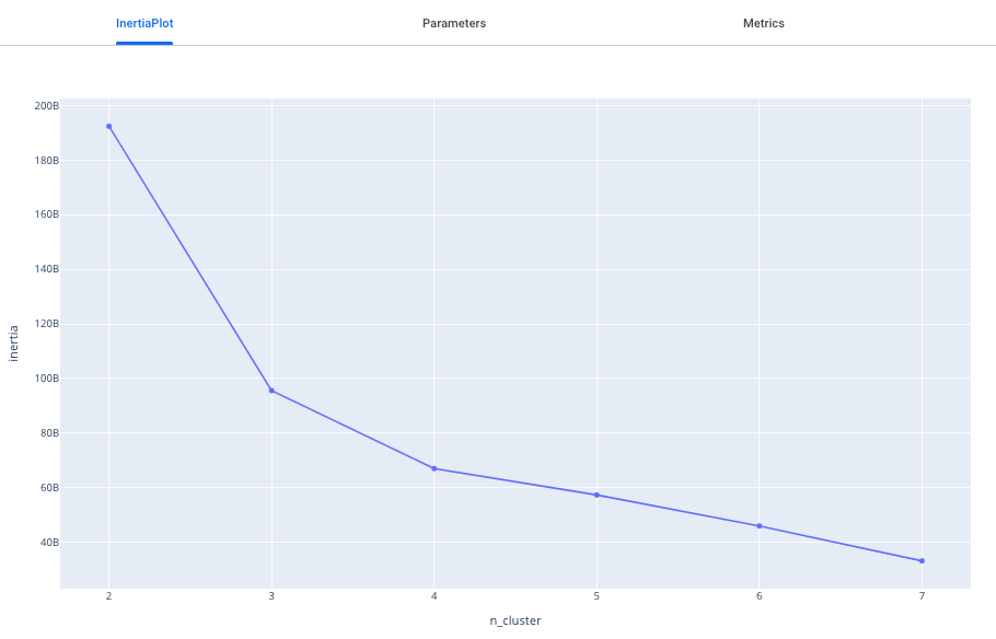
How many optimal groups can the data points be categorized into?
In the current scenario, based on the below plot, we can have 3 groups.
What are the main features we should consider for the grouping?
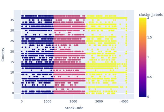
The above plot indicates that stockcode and country should be considered as the main features while grouping to make business decisions.
Acting on Insights
Section titled “Acting on Insights”Both enriched data and customer segmentation information can be sent to target systems to operationalize insights. This data can be saved to a destination, such as an S3 bucket, as a new file for downstream use.
Business Case 4 (Time Series): Store Sales Data
Section titled “Business Case 4 (Time Series): Store Sales Data”A store would like to analyze and forecast sales trends to improve decision-making for store operations and marketing. Understanding sales dynamics is critical for effective inventory management, planning promotions, and predicting future sales performance. The primary focus of this analysis is to determine whether the data is stationary, identify trends or seasonal patterns, and explore peak sales periods while forecasting future sales.
The ARIMA time series model is employed to forecast future sales while accounting for these trends and patterns. ARIMA is chosen for its ability to handle both autoregressive (AR) and moving average (MA) components while incorporating differencing to make the data stationary.
Dataset Overview
Section titled “Dataset Overview”You can download the Store Sales Time Series Data from Kaggle.
Here, the store captures sales of products. The dataset gives the sales over the span of 8 years. This is a small dataset with no null values.
Analysis Questions:
- Is data stationary?
- Does it have trend or seasonality?
- What are the peak sales periods? ***
- What’s the overall sales growth trend? ***
- Are there clear seasonal patterns in sales? ***
*** Note: This entails advanced techniques that will be addressed in the Data Science Handbook. For now, the assumption is that these reports are available for analysis.
Importing Data
Section titled “Importing Data”Understanding the Data
Section titled “Understanding the Data”Once the data is imported, create a dataset for enrichment purposes. Data exploration (suggested checklist) — the Store Sales dataset tracks the number of transactions on a given day. There are no missing values in this dataset.
xVector provides out-of-the-box tools to profile the data. Generate Exploratory Report and Generate Report are GenAI reports built on the platform.
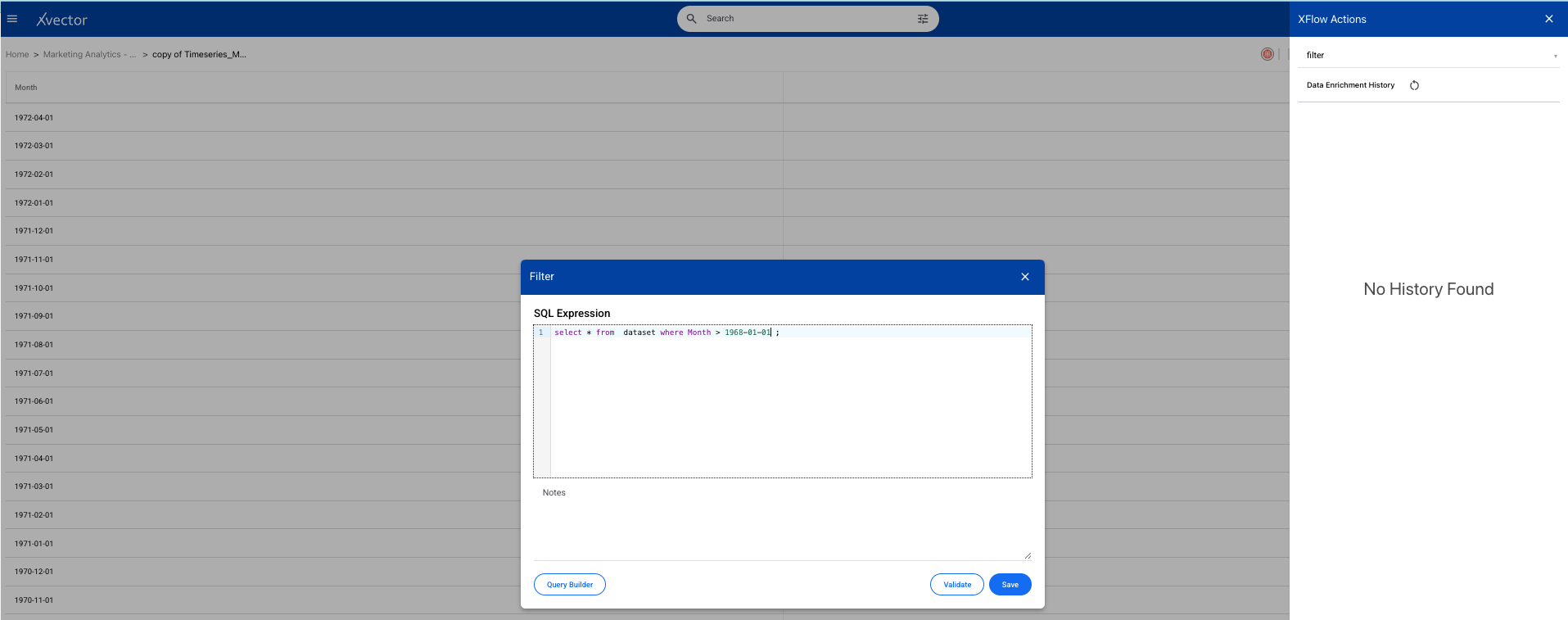
Once you perform basic exploration of the data, you can then enrich the data. For example, “filter” is one such function used to filter appropriate records.
Forecasting Sales Trends
Section titled “Forecasting Sales Trends”For the current dataset, we will use an existing model driver, stats_ARIMA. Follow the steps to build a time series model and use the model stats_ARIMA. Use appropriate parameters and evaluation metrics to optimize the solution.
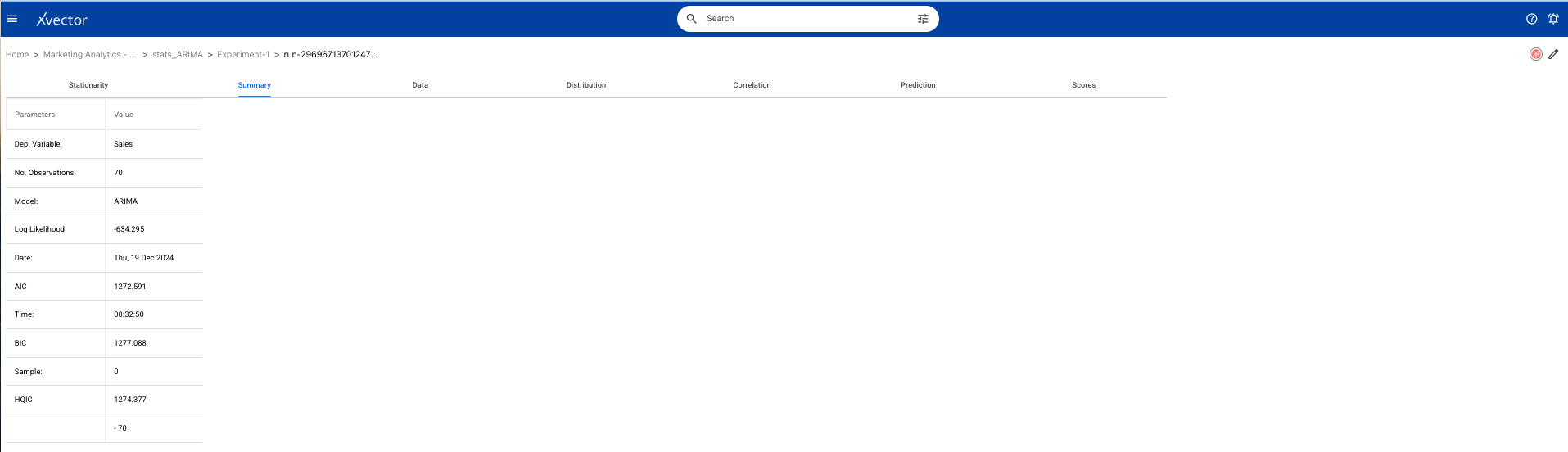
Here is a time series model implemented in xVector.
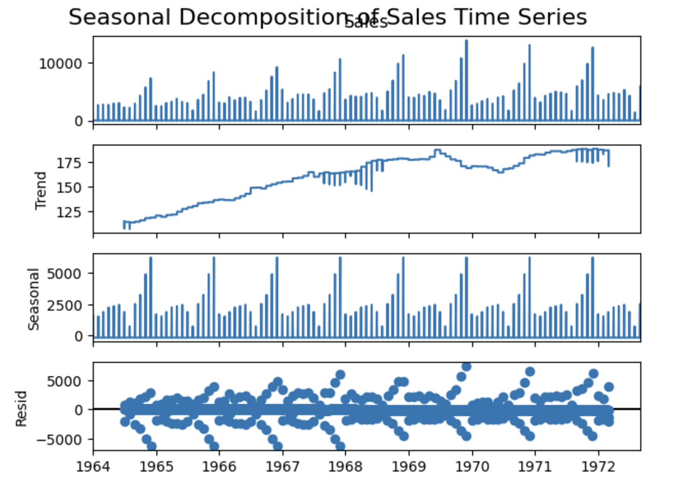
Analysis
Section titled “Analysis”Is data stationary?
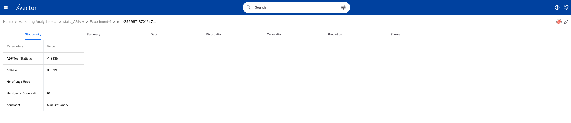
Based on the above analysis, the dataset is non-stationary. This implies that the data shows trends, seasonality, or varying variance over time.
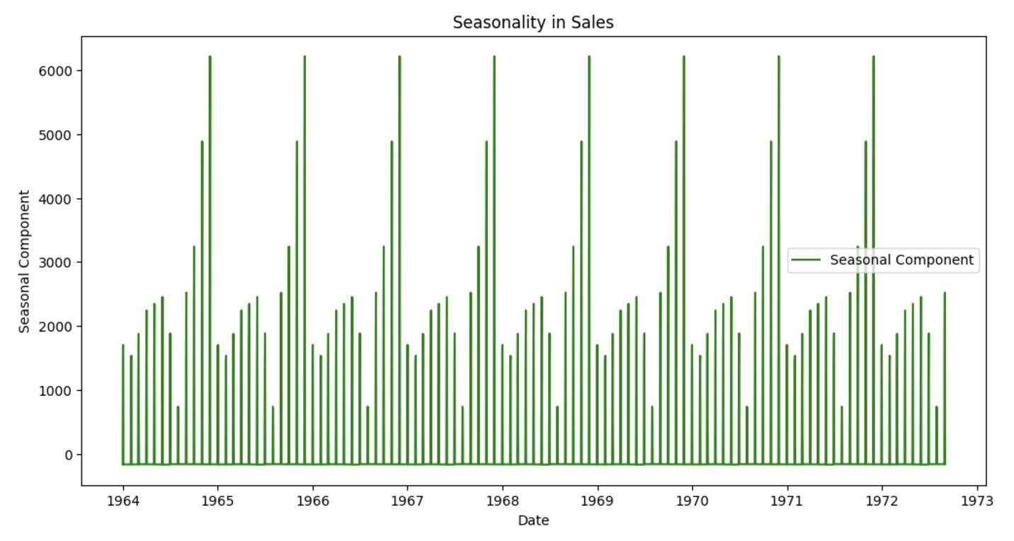
Does it have trend or seasonality?
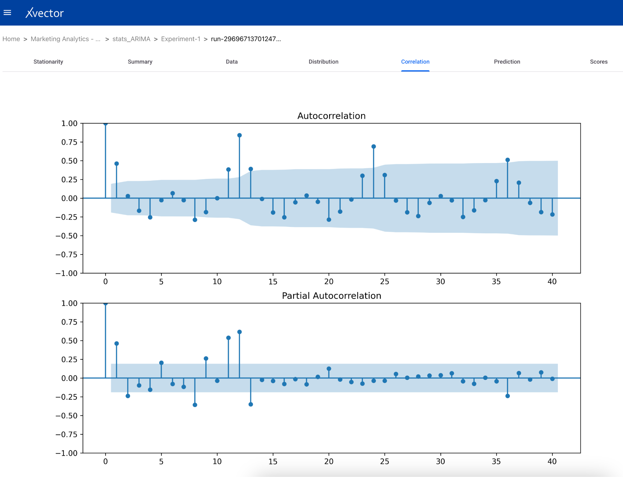
The autocorrelation function (ACF) and partial autocorrelation function (PACF) plots help in understanding the temporal dependencies in the data. If the ACF plot shows a slow decay, this suggests the presence of a trend. If you notice spikes at regular intervals, this indicates the presence of seasonality — suggesting the need for seasonal differencing or a SARIMA model.
**What are the peak sales periods? *****
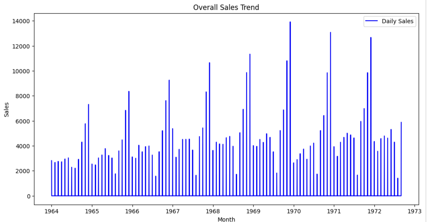
December of every year has peak sales.
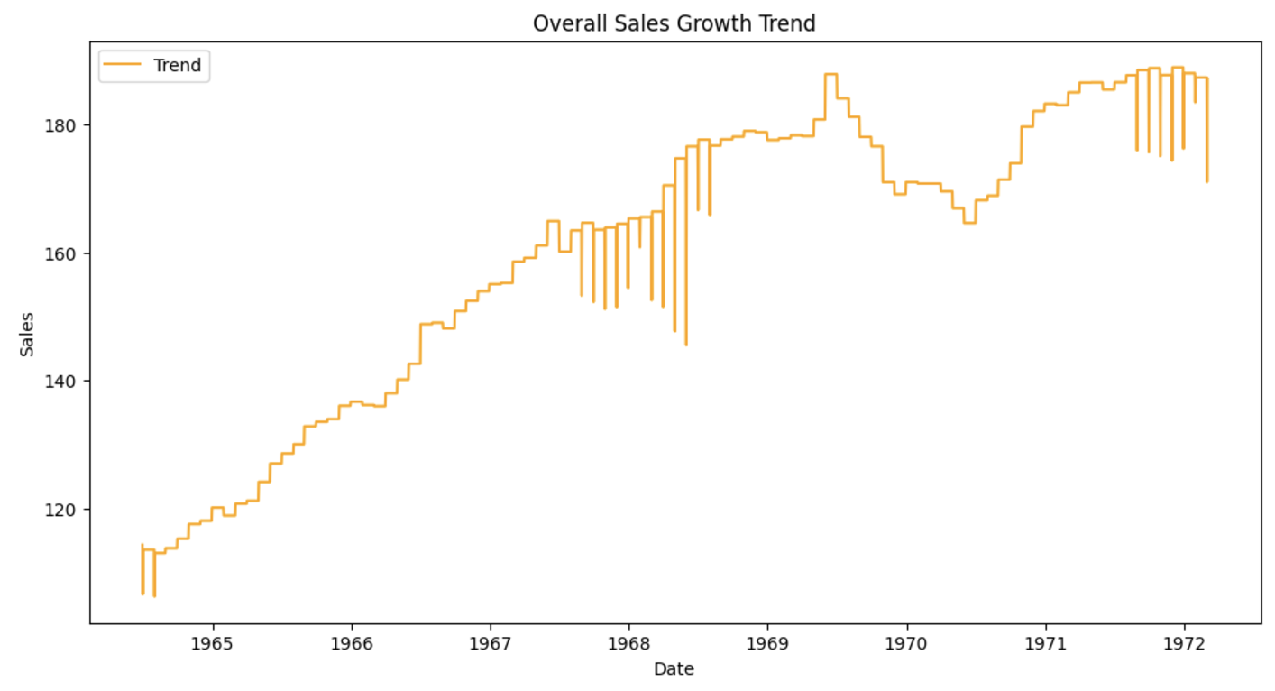
**What’s the overall sales growth trend? *****
**Are there clear seasonal patterns in sales? *****
- Holiday Patterns: Sales peak in December (holiday season) and November (Black Friday).
- Long-Term Trends: Seasonal patterns might change over time, indicating shifting consumer behavior.
- Overall Growth: The trend component reveals whether the store’s sales are growing, stagnating, or declining.
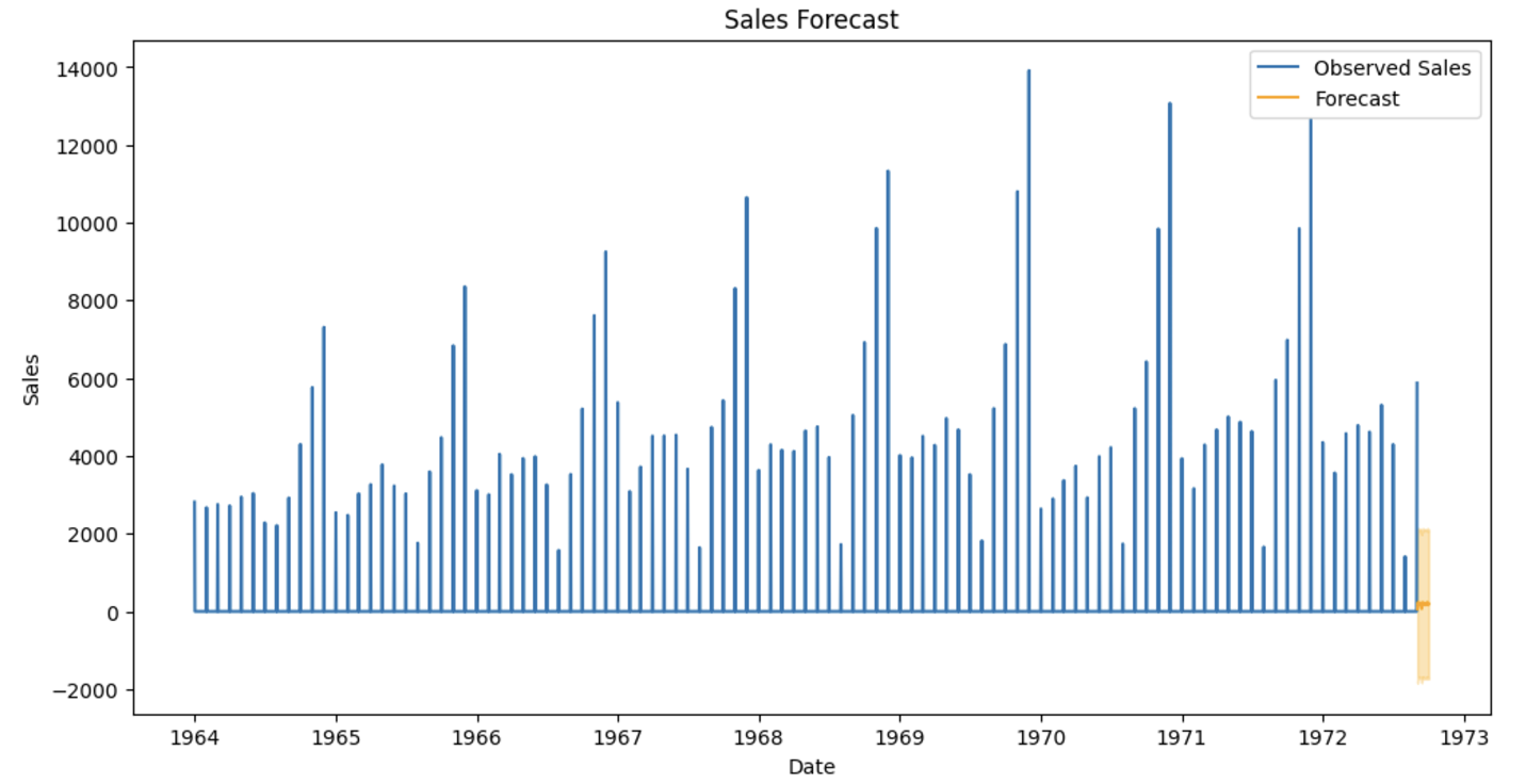
Sales forecast:
Appendix
Section titled “Appendix”Typical Data Analysis Process
Section titled “Typical Data Analysis Process”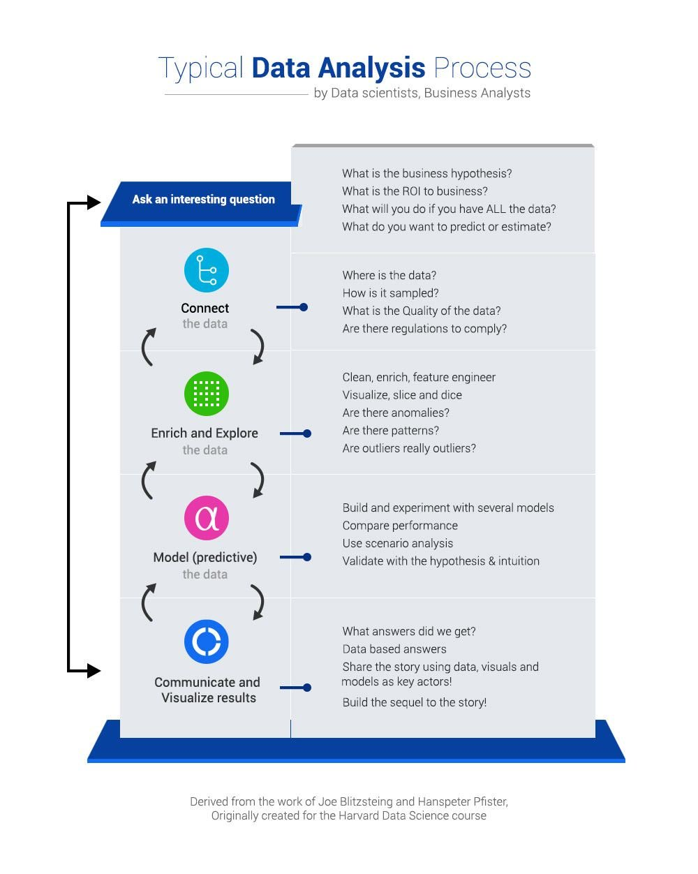
Sample Data Exploration Checklist
Section titled “Sample Data Exploration Checklist”Exploring data (often called Exploratory Data Analysis or EDA) is a critical process of examining and understanding a dataset before diving into formal modeling.
Context & Source — What business process/system generated the data? What is the purpose of collecting this data? What is the unit of observation (row = transaction, customer etc.)? What is the time coverage (start & end dates)? Are there known biases?
Data Quality — Are there missing values? Duplicate records? Are numeric values within expected ranges? Are categorical values standardized (e.g., “FB” vs. “Facebook”)? Are timestamps correctly formatted? Are there anomalies (e.g., negative revenue, invalid dates)?
Data Structure — What are the data types (numeric, categorical, text, datetime)? Which fields can serve as keys or identifiers? How many records and features? What’s the distribution of key numeric fields? What’s the frequency of categorical values?
Behavior & Relationships — Are there trends over time? Correlations between key variables? Outliers that may distort the analysis? Have the statistical properties of data changed over time (data drift)?
Visualization Techniques — Histograms for data distribution, box plots for spread and outliers, scatter plots for relationships, correlation matrices for feature interactions, heat maps for complex patterns.
Selecting Appropriate Chart
Section titled “Selecting Appropriate Chart”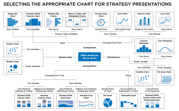
Linear Regression: Parameters and Evaluating Metrics
Section titled “Linear Regression: Parameters and Evaluating Metrics”Parameters
Parameters are the configurable settings and learned values that define how a machine learning model operates and makes predictions. They control the model’s complexity, learning behavior, and decision-making process. Proper parameter selection and tuning are crucial for model performance, as they directly influence the model’s ability to generalize to new, unseen data.
Scikit-learn provides details of the parameters for Linear Regression model.
| Model | Parameter | Description | Usage |
|---|---|---|---|
| Linear Regression | fit_intercept | Whether to calculate the intercept for the regression model | Set False if the data is already centered |
| normalize | Normalizes input features. Deprecated in recent Scikit-learn versions | Helps with features on different scales | |
| test_size | Size of test data | Helps with splitting train and test data | |
| Ridge Regression | alpha | L2 regularization strength. Larger values shrink coefficients more | Prevents overfitting by reducing model complexity |
| solver | Optimization algorithm: auto, saga, etc. | Impacts convergence speed and stability for large datasets | |
| Lasso Regression | alpha | L1 regularization strength. Controls sparsity of coefficients | Useful for feature selection |
| max_iter | Maximum iterations for optimization | Impacts convergence for large or complex datasets | |
| XGBoost (Regression) | eta (learning rate) | Step size for updating predictions | Lower values make learning slower but more robust |
| max_depth | Maximum depth of trees | Higher values can capture complex relationships but risk overfitting | |
| colsample_bytree | Fraction of features sampled for each tree | Introduces randomness, reducing overfitting |
Evaluating Metrics
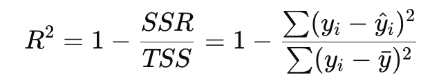
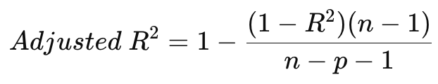
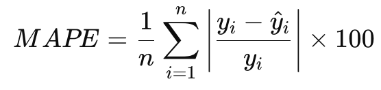
Regression models predict continuous values, so the metrics focus on measuring the difference between predicted and actual values.
In the formulas below: n = number of observations, ŷ = predicted value, y = actual value, SSR = Sum of Squares Regression, TSS = Total Sum of Squares.
| Metric | Description |
|---|---|
| Mean Absolute Error (MAE) | Measures the average magnitude of errors without considering their direction. A lower MAE indicates better model performance. It’s easy to interpret but doesn’t penalize large errors as much as MSE. |
| Mean Squared Error (MSE) | Computes the average squared difference between actual and predicted values. Penalizes larger errors more than MAE, making it sensitive to outliers. |
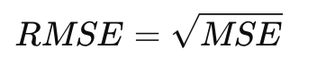
| Root Mean Squared Error (RMSE) | Square root of MSE; represents errors in the same unit as the target variable. Balances interpretability and sensitivity to large errors. |
| R² Score (Coefficient of Determination) | Proportion of variance explained by the model. Values range from 0 to 1, where 1 means perfect prediction. Negative values indicate poor performance. |
| Adjusted R² | Adjusts R² for the number of predictors in the model, by penalizing the addition of irrelevant features. Useful for comparing models with different numbers of predictors. |
| Mean Absolute Percentage Error (MAPE) | Measures error as a percentage of actual values, making it scale-independent. Useful for scale-independent evaluation but struggles with very small actual values. |
Formulas:
MAE:
MSE:
RMSE:
R² Score:
Adjusted R²:
MAPE:
Classification: Parameters and Evaluating Metrics
Section titled “Classification: Parameters and Evaluating Metrics”Parameters
Parameters are the configurable settings and learned values that define how a machine learning model operates and makes predictions. They control the model’s complexity, learning behavior, and decision-making process. Proper parameter selection and tuning are crucial for model performance, as they directly influence the model’s ability to generalize to new, unseen data.
Scikit-learn provides details of the parameters for Random Forest Classification model.
| Model | Parameter | Description | Usage |
|---|---|---|---|
| Random Forest Classifier | n_estimators | Number of trees in the forest | Affects accuracy and training speed; larger forests usually perform better |
| max_features | Number of features to consider when splitting | Reduces overfitting and speeds up training | |
| bootstrap | Whether to sample data with replacement | Improves diversity among trees | |
| Logistic Regression | penalty | Type of regularization: l1, l2, elasticnet, or none | Adds constraints to model coefficients to prevent overfitting |
| solver | Optimization algorithm: liblinear, saga, lbfgs, etc. | Determines how the model is optimized, with some solvers supporting specific penalties | |
| C | Inverse of regularization strength. Smaller values increase regularization | Balances bias and variance | |
| max_iter | Maximum number of iterations for optimization | Ensures convergence for complex problems | |
| Support Vector Machine (SVM) | C | Regularization parameter. Smaller values create larger margins but may underfit | Controls the trade-off between misclassification and margin size |
| kernel | Kernel type: linear, rbf, poly, or sigmoid | Determines how data is transformed into higher dimensions | |
| gamma | Kernel coefficient for non-linear kernels | Impacts the decision boundary for non-linear kernels like rbf or poly | |
| Decision Tree Classifier | criterion | Function to measure split quality: gini or entropy | Controls how splits are chosen (impurity vs. information gain) |
| max_depth | Maximum depth of the tree | Prevents overfitting by restricting the complexity of the tree | |
| min_samples_split | Minimum samples required to split a node | Ensures that nodes are not split with very few samples | |
| min_samples_leaf | Minimum samples required in a leaf node | Prevents overfitting by ensuring leaves have sufficient data | |
| K-Nearest Neighbors (KNN) | n_neighbors | Number of neighbors to consider for classification | Affects granularity of classification; smaller values lead to more localized decisions |
| weights | Weighting function: uniform (equal weight) or distance (closer points have higher weight) | Impacts how neighbors influence the prediction | |
| metric | Distance metric: minkowski, euclidean, manhattan, etc. | Defines how distances between data points are calculated | |
| Naive Bayes | var_smoothing | Portion of variance added to stabilize calculations | Prevents division by zero for features with very low variance |
| XGBoost (Classification) | objective | Specifies the learning task: binary:logistic, multi:softprob, etc. | Matches the classification type (binary or multiclass) |
| scale_pos_weight | Balances positive and negative classes for imbalanced datasets | Essential for tasks like fraud detection where class imbalance is significant | |
| max_depth | Maximum depth of trees | Higher values increase model complexity but risk overfitting | |
| eta (learning rate) | Step size for updating predictions | Smaller values lead to slower, more accurate training | |
| gamma | Minimum loss reduction required for further tree splits | Higher values make the model more conservative |
Evaluating Metrics
Classification models predict discrete labels, so the metrics measure the correctness of those predictions.
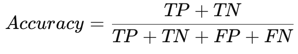
In the formulas below: TP = True Positives, TN = True Negatives, FP = False Positives, FN = False Negatives.
| Metric | Description |
|---|---|
| Accuracy | Ratio of correct predictions to total predictions. Works well for balanced datasets but fails for imbalanced ones. |
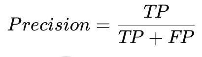
| Precision | Fraction of true positive predictions among all positive predictions. High precision minimizes false positives. |
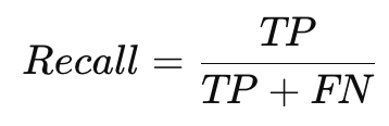
| Recall (Sensitivity) | Fraction of actual positives that were correctly predicted. High recall minimizes false negatives. |
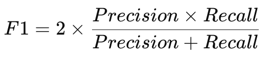
| F1 Score | Harmonic mean of precision and recall. Best suited for imbalanced datasets. |
| Confusion Matrix | Tabular representation of true positives, true negatives, false positives, and false negatives. Helps visualize classification performance. |
| ROC-AUC Score | Measures the trade-off between true positive rate (TPR) and false positive rate (FPR). Evaluates a classifier’s ability to distinguish between classes at various thresholds. Higher AUC indicates better performance. |
Formulas:
Accuracy:
Precision:
Recall:
F1 Score:
Clustering: Parameters and Evaluating Metrics
Section titled “Clustering: Parameters and Evaluating Metrics”Parameters
Parameters are the configurable settings and learned values that define how a machine learning model operates and makes predictions. They control the model’s complexity, learning behavior, and decision-making process. Proper parameter selection and tuning are crucial for model performance, as they directly influence the model’s ability to generalize to new, unseen data.
Scikit-learn provides details of the parameters for KMeans clustering.
| Model | Parameter | Description | Usage |
|---|---|---|---|
| K-Means | n_clusters | Number of clusters to form | Controls the number of groups/clusters in the data |
| init | Initialization method for centroids: k-means++, random | k-means++ is better for convergence | |
| max_iter | Maximum number of iterations to run the algorithm | Prevents infinite loops and ensures convergence | |
| tol | Tolerance for convergence | Stops the algorithm when the centroids’ movement is smaller than this value | |
| n_init | Number of times the K-Means algorithm will be run with different centroid seeds | Ensures better centroids and better performance | |
| DBSCAN | eps | Maximum distance between two points to be considered neighbors | Determines cluster density |
| min_samples | Minimum number of points required to form a dense region (a cluster) | Larger values lead to fewer but denser clusters | |
| metric | Distance metric used for clustering: euclidean, manhattan, etc. | Affects the way distances are calculated between points | |
| Agglomerative Clustering | n_clusters | Number of clusters to form | Specifies the number of clusters to form at the end of the clustering process |
| linkage | Determines how to merge clusters: ward, complete, average, or single | Affects how clusters are combined (Ward minimizes variance) | |
| affinity | Metric used to compute distances: euclidean, manhattan, cosine, etc. | Affects the distance measure between data points during clustering | |
| K-Medoids | n_clusters | Number of clusters to form | Specifies the number of clusters (like K-Means but uses medoids) |
| metric | Distance metric for pairwise dissimilarity | Defines the method for calculating pairwise distances between points | |
| max_iter | Maximum number of iterations to run the algorithm | Ensures termination after a certain number of iterations | |
| Gaussian Mixture Model | n_components | Number of mixture components (clusters) | Determines the number of Gaussian distributions (clusters) |
| covariance_type | Type of covariance matrix: full, tied, diag, or spherical | Defines how the covariance of the components is calculated | |
| tol | Convergence threshold | Stops iteration if log-likelihood change is smaller than tol | |
| max_iter | Maximum number of iterations for the EM algorithm | Ensures the algorithm stops after a fixed number of iterations |
Evaluating Metrics
Clustering models are unsupervised, so metrics evaluate the quality of the clusters formed.
| Metric | Description |
|---|---|
| Silhouette Score | Measures how well clusters are separated and how close points are within a cluster. Ranges from -1 to 1. Higher values indicate well-separated and compact clusters. |
| Davies-Bouldin Index | Measures the average similarity ratio of each cluster with the most similar cluster. It measures intra-cluster similarity relative to inter-cluster separation. Lower is better. Evaluates compactness and separation of clusters. |
| Calinski-Harabasz Score | Ratio of cluster separation to cluster compactness. Higher values indicate better-defined clusters. |
| Adjusted Rand Index (ARI) | Compares the clustering result to a ground truth (if available). Adjusts for chance clustering. |
| Mutual Information Score | Measures agreement between predicted clusters and ground truth labels. Higher values indicate better alignment. |
Timeseries: Parameters and Evaluating Metrics
Section titled “Timeseries: Parameters and Evaluating Metrics”Parameters
Parameters are the configurable settings and learned values that define how a machine learning model operates and makes predictions. They control the model’s complexity, learning behavior, and decision-making process. Proper parameter selection and tuning are crucial for model performance, as they directly influence the model’s ability to generalize to new, unseen data.
Scikit-learn provides details of the parameters for ARIMA Timeseries.
| Model | Parameter | Description | Usage |
|---|---|---|---|
| ARIMA | p | Number of lag observations (autoregressive part) | Captures dependency on past values |
| d | Degree of differencing to make the series stationary | Removes trends from the data | |
| q | Number of lagged forecast errors (moving average part) | Models dependency on past prediction errors | |
| SARIMA | seasonal_order | Tuple (P, D, Q, m) where m is the season length | Adds seasonal components to ARIMA |
| trend | Specifies long-term trend behavior: n (none), c (constant), or t (linear) | Helps model global trends in data | |
| weekly_seasonality | Whether to include weekly seasonality (True/False or int for harmonics) | Useful for datasets with strong weekly patterns like retail sales | |
| XGBoost (for Time Series) | max_depth | Maximum depth of trees used for feature-based time series modeling | Captures complex temporal relationships |
| eta (learning rate) | Step size for updating predictions in gradient boosting | Lower values improve robustness but require more iterations | |
| colsample_bytree | Fraction of features sampled for each tree | Reduces overfitting and adds diversity | |
| subsample | Fraction of training instances sampled for each boosting iteration | Introduces randomness to prevent overfitting | |
| objective | Learning task, e.g., reg:squarederror for regression tasks | Matches the regression nature of time series forecasting | |
| lambda | L2 regularization term on weights | Controls overfitting by penalizing large coefficients | |
| alpha | L1 regularization term on weights | Adds sparsity, which is helpful for feature selection | |
| booster | Type of booster: gbtree, gblinear, or dart | Tree-based (gbtree) is most common for time series | |
| LSTM | units | Number of neurons in each LSTM layer | Higher values increase model capacity but risk overfitting |
| input_shape | Shape of input data (timesteps, features) | Specifies the window of historical data and number of features | |
| return_sequences | Whether to return the full sequence (True) or the last output (False) | Use True for stacked LSTMs or sequence outputs | |
| dropout | Fraction of neurons randomly dropped during training (e.g., 0.2) | Prevents overfitting by adding regularization | |
| recurrent_dropout | Fraction of recurrent connections dropped during training | Adds regularization to the temporal dependencies | |
| optimizer | Algorithm for adjusting weights (e.g., adam, sgd) | Controls how the model learns from errors | |
| loss | Loss function (e.g., mse, mae, huber) | Determines how prediction errors are minimized | |
| batch_size | Number of sequences processed together during training | Smaller batches generalize better but take longer to train | |
| epochs | Number of complete passes over the training dataset | Too many epochs may lead to overfitting | |
| timesteps | Number of past observations used to predict future values | Determines the window of historical data analyzed for prediction | |
| Orbit | response_col | Name of the column containing the target variable (e.g., sales) | Specifies which variable is being forecasted |
| date_col | Name of the column containing dates | Identifies the time index for forecasting | |
| seasonality | Seasonal periods (e.g., weekly, monthly, yearly) | Models seasonality explicitly, crucial for periodic patterns in time-series data | |
| seasonality_sm_input | Number of Fourier terms used for seasonality approximation | Controls the smoothness of seasonality; higher values increase granularity | |
| level_sm_input | Smoothing parameter for the level component (between 0 and 1) | Determines how quickly the model adapts to recent changes in level | |
| growth_sm_input | Smoothing parameter for the growth component | Adjusts the sensitivity of the growth trend over time | |
| estimator | Optimizer used for parameter estimation (stan-map, pyro-svi, etc.) | stan-map for faster optimization, pyro-svi for full Bayesian inference | |
| prediction_percentiles | Percentiles for the uncertainty intervals (default: [5, 95]) | Defines the confidence intervals for forecasts | |
| num_warmup | Number of warmup steps in sampling (used in Bayesian methods) | Higher values improve parameter estimation but increase computation time | |
| num_samples | Number of posterior samples drawn (used in Bayesian methods) | Ensures good posterior estimates; higher values yield more robust uncertainty estimates | |
| regressor_col | Name(s) of columns used as regressors | Incorporates additional covariates into the model (e.g., holidays, promotions) |
Evaluating Metrics
Time series models focus on predicting sequential data, so metrics measure the alignment of predicted values with the observed trend. In addition to MAE, MSE, RMSE, and MAPE (see formulas above):
| Metric | Description |
|---|---|
| Mean Absolute Error (MAE) | See regression metrics above |
| Mean Squared Error (MSE) | See regression metrics above. Penalizes larger errors more than MAE, making it sensitive to outliers in time series. |
| Root Mean Squared Error (RMSE) | See regression metrics above. Evaluates prediction accuracy in the original scale of the data. |
| Mean Absolute Percentage Error (MAPE) | See regression metrics above. Useful for scale-independent evaluation but struggles with very small actual values. |
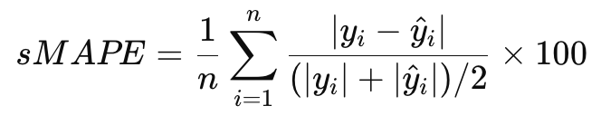
| Symmetric Mean Absolute Percentage Error (sMAPE) | Variant of MAPE, mitigates issues with small denominators. |
| Dynamic Time Warping (DTW) | Measures similarity between two time series, even if they are misaligned. |
| R² Score | Evaluates variance explained by the time series model. |
sMAPE Formula:
Model Comparison
Section titled “Model Comparison”| Aspect | Regression | Classification | Clustering | Time Series |
|---|---|---|---|---|
| Purpose | Predicts continuous values | Assigns to categories | Groups by similarity | Predicts future values |
| Output | Continuous (e.g., prices) | Labels (e.g., spam/not) | Cluster labels | Future predictions |
| Learning | Supervised | Supervised | Unsupervised | Supervised/Unsupervised |
| Algorithms | Linear, Gradient Boosting | Logistic, Random Forest, SVM | K-Means, DBSCAN | ARIMA, LSTM, Prophet |
| Use Cases | Price/sales prediction | Fraud detection, diagnosis | Customer segmentation | Sales/traffic forecasting |
A Few Learning Principles
Section titled “A Few Learning Principles”These principles are taken from “Learning from data”, a Caltech course by Yaser Abu-Mostafa: https://work.caltech.edu/telecourse
Occam’s Razor — Prefer simpler models that adequately fit the data to reduce overfitting.
Bias and Variance — Bias is error from oversimplifying (underfitting). Variance is error from overcomplexity (overfitting). A good model balances both. High Variance signs: training MSE low but test MSE much higher. High Bias signs: both training and test MSE are high.
Data Snooping — Avoid tailoring models too closely to specific datasets through repeated testing. Prevent it by separating data properly, using k-fold cross-validation, performing feature engineering only on training data, keeping a final holdout set untouched, and documenting data usage transparently.
References
Section titled “References”- Learning From Data - Caltech
- Kaggle Learn
- Encoding Categorical Data in SkLearn
- Analyst Academy
- Data Science for Marketing Analytics — By Tommy Blanchard, Debasish Behera, Pranshu Bhatnagar
- Applied Machine Learning in Python — By Professor Michael J. Pyrcz